Transformers and Self-Attention
Table of Contents:
- Overview
- Limitations of MLPs
- Intuition Behind Attention
- Masked Self-Attention + Implementation
- Cross Attention
- Feedforward Layer + Implementation
- Tokenization and Positional Encoding
- Encoder-Decoder vs. Encoder-Only vs. Decoder-Only
- Perceiver Architecture
- Vision Transformer
Overview
Understanding recent works in ML isn’t possible without a deep understanding of how Transformers work. They represent the SOTA in every AI field – computer vision, NLP, speech, machine translation, RL, robotics, and more. Over the past several years, several excellent resources on Transformers have come to light from Andrej Karpathy, Lucas Beyer, Dmitry Kobak, and Jay Mody. This post is my attempt to synthesize the best resources out there. This will put Transformers in the context of existing tools, such as MLPs and RNNs. We’ll implement each aspect of a Transformer in Python, step by step. Transformers are a special case of graph neural networks (GNNs), as a nice post illustrates.
Transformer architectures interleaves attention layers with MLP layers. Importantly, each module’s output has the exact same shape as its input. We’ll start with discussing the intuition behind the attention operation.
On the Limitations of MLPs
Problem Definition Suppose we have a text string, split into tokens (sequence length \(T \leq 512\)). Each token gets a \(C=768\)-dim vector. So we have a 2D matrix \(X \in \mathbb{R}^{768 \times 512}\) of arbitrary width (this is the BERT / GPT setting).
Why are MLPs insufficient? Suppose we want to set up a feed-forward layer that would somehow transform \(X\), keeping its shape. A fully-connected layer does not work: it cannot take input of variable length (and would have too many params anyway even if we padded). If we didn’t flatten it, we would be only acting on the embedding dimension, which would process each token separately, which is clearly not sufficient. To make the tokens interact, we would need to flatten it, getting \((512 \cdot 768)^2 = 154\)B params (far too many).
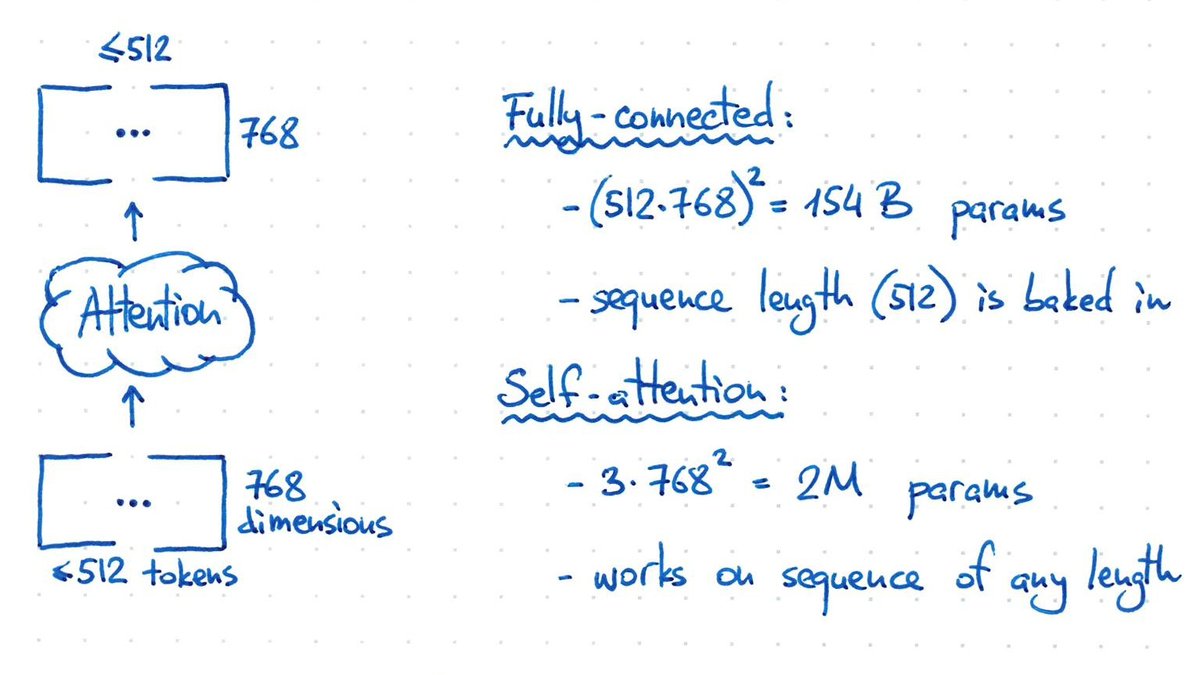
If we act only on the embedding dimension, we’ll ignore the batch dimension, which would be a single leading dimension on \(X\), and doesn’t affect the intuition behind attention in any way.
# MLP, w/ no interaction!
import numpy as np
T = 512
C = 768
X = np.random.randn(C, T)
W = np.random.randn(C, C)
# (C_out=C, C) @ (C, T)
out = W @ X
>>> out.shape
# (C=768, T=512)
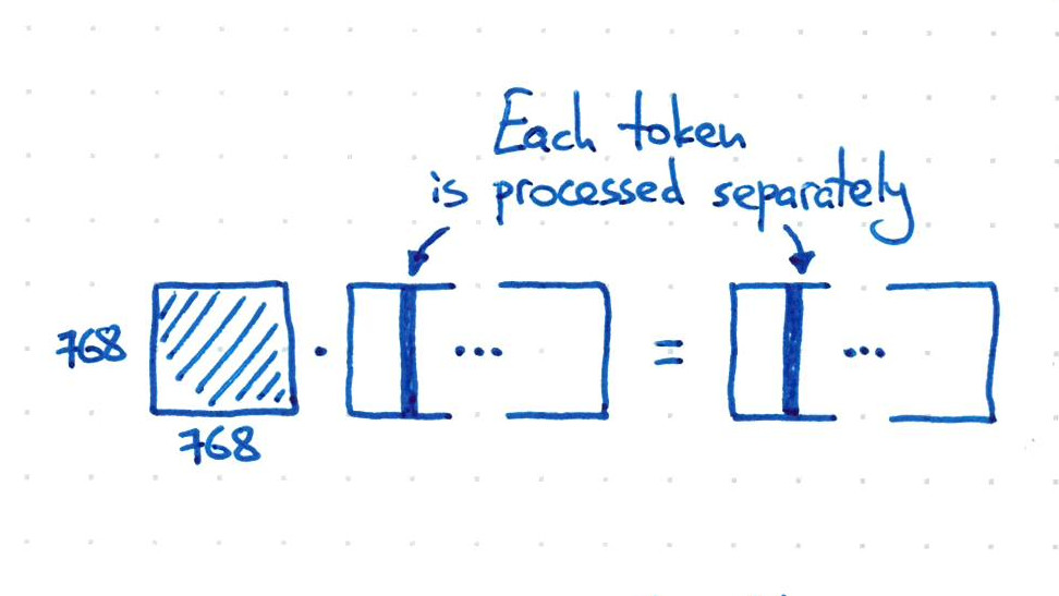
We could get interaction via flattening, but run out of memory from the 154B params:
# MLP, w/ interaction (by flattening)!
X = np.random.randn(T, C).reshape(T * C)
W = np.random.randn(T * C, T * C)
# (C_out=T*C, T*C) @ (T*C, 1)
out = W @ X
>>> out.shape
# (T*C = 512*768)
Intuition Behind Attention
To design the attention operation, the key question we wish to answer is, how can we make the tokens interact, using fewer parameters, for variable sequence lengths?
X @ X.T @ X has the correct output shape, with full interaction, (C, T) * (T, C) * (C, T) = (C, T), but no learnable params.
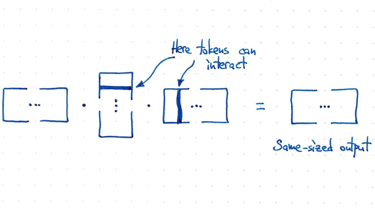
This can be thought of as \(V(K^TQ)\), a transposed version of the essential Vaswani et al. Transformer equation: \(\mbox{softmax}(\frac{QK^T}{\sqrt{d_{key}}}) V\), since we used the transposed input notation \(X \in \mathbb{R}^{C \times T}\) instead of \(X \in \mathbb{R}^{T \times C}\).
Of course we want learned params, so if we stick a learned matrix in the middle, a learned interaction can be implemented as:
# Self-attention, w/ interaction.
X = np.random.randn(C, T)
W = np.random.randn(C, C)
V = np.random.randn(C, C)

(X.T @ W @ X).shape
# (T=512, T=512)

X @ (X.T @ W @ X).shape
# (C=768, T=512)

out = (V @ X) @ (X.T @ W @ X)
out.shape
# (C=768, T=512)
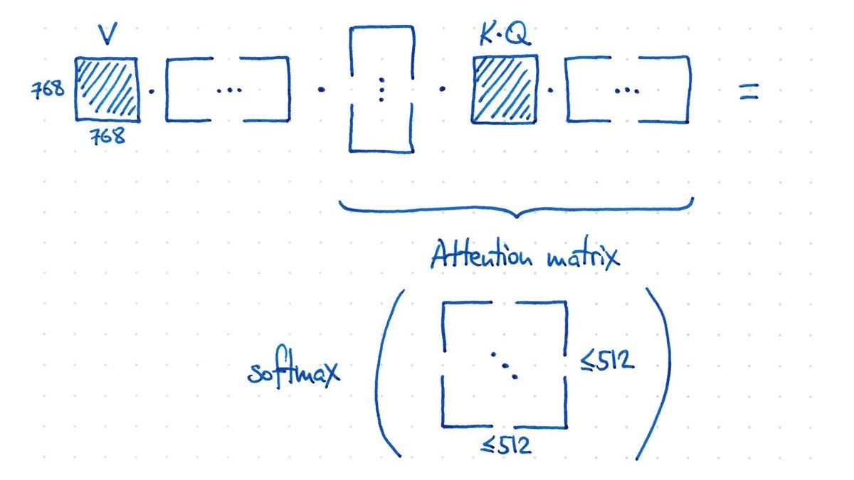
Each token can “look around” the whole input, and decide how to update its representation based on what it sees.
Self-Attention Implementation
Attention is a topic that only makes sense through code examples, so we’ll work through one together. We’ll train a BiGram model, from Karpathy’s very useful GPT Colab. We’ll use text as toy data for the model.
Specifically, we’ll use the Tiny Shakespeare Dataset consisting of 1.1M characters:
# let's look at the first 1000 characters
print(text[:1000])
# First Citizen:
# Before we proceed any further, hear me speak.

# All:
# Speak, speak.

# First Citizen:
# You are all resolved rather to die than to famish?
...
A 65-character vocabulary will capture the whole text. Note that it includes ‘\n’ and ‘ ‘:
# here are all the unique characters that occur in this text
chars = sorted(list(set(text)))
vocab_size = len(chars)
print(''.join(chars))
print(vocab_size)
#
#  !$&',-.3:;?ABCDEFGHIJKLMNOPQRSTUVWXYZabcdefghijklmnopqrstuvwxyz
# 65
Next, let’s create a mapping from characters to integers, and back again:
stoi = { ch:i for i,ch in enumerate(chars) }
itos = { i:ch for i,ch in enumerate(chars) }
encode = lambda s: [stoi[c] for c in s] # encoder: take a string, output a list of integers
decode = lambda l: ''.join([itos[i] for i in l]) # decoder: take a list of integers, output a string

print(encode("hii there"))
print(decode(encode("hii there")))
# [46, 47, 47, 1, 58, 46, 43, 56, 43]
# hii there
Let’s now encode the entire text dataset and store it into a torch.Tensor:
import torch # we use PyTorch: https://pytorch.org
data = torch.tensor(encode(text), dtype=torch.long)
print(data.shape, data.dtype)
print(data[:1000]) # the 1000 characters we looked at earier will to the GPT look like this
# torch.Size([1115394]) torch.int64
# tensor([18, 47, 56, 57, 58,  1, 15, 47, 58, 47, 64, 43, 52, 10,  0, 14,
#         43, 44, 53, 56, 43,  1, 61, 43,  1, 54, 56, 53, 41, 43, 43, 42, ...
Let’s now split up the data into train and validation sets
n = int(0.9*len(data)) # first 90% will be train, rest val
train_data = data[:n]
val_data = data[n:]
# n = 1003854
Transformers condition on the past using a “context window”. We’ll define its length as block_size:
block_size = 8
x = train_data[:block_size]
y = train_data[1:block_size+1]
for t in range(block_size):
    context = x[:t+1]
    target = y[t]
    print(f"when input is {context} the target: {target}")
# when input is tensor([18]) the target: 47
# when input is tensor([18, 47]) the target: 56
# when input is tensor([18, 47, 56]) the target: 57
# when input is tensor([18, 47, 56, 57]) the target: 58
# when input is tensor([18, 47, 56, 57, 58]) the target: 1
# when input is tensor([18, 47, 56, 57, 58,  1]) the target: 15
# when input is tensor([18, 47, 56, 57, 58,  1, 15]) the target: 47
# when input is tensor([18, 47, 56, 57, 58,  1, 15, 47]) the target: 58
from typing import Tuple

torch.manual_seed(1337)
batch_size = 4 # how many independent sequences will we process in parallel?
block_size = 8 # what is the maximum context length for predictions?

def get_batch(split: str) -> Tuple[torch.Tensor, torch.Tensor]:
    # Generate a small batch of data of inputs `x` and targets `y`.
    data = train_data if split == 'train' else val_data
    ix = torch.randint(high=len(data) - block_size, size=(batch_size,))
    # shape: (batch_size, block_size).
    x = torch.stack([data[i:i+block_size] for i in ix])
    y = torch.stack([data[i+1:i+block_size+1] for i in ix])
    return x, y
In LLaMA 1, 2, 3, the block_size (context window length) is 2048, 4096, and 128K tokens, respectively.
xb is our input to the transformer
xb, yb = get_batch(split='train')
print('inputs:')
print("xb shape: ", xb.shape)
print(xb)
print('targets:')
print("yb shape: ", yb.shape)
print(yb)
# inputs:
# xb shape:  torch.Size([4, 8])
# tensor([[24, 43, 58,  5, 57,  1, 46, 43],
#         [44, 53, 56,  1, 58, 46, 39, 58],
#         [52, 58,  1, 58, 46, 39, 58,  1],
#         [25, 17, 27, 10,  0, 21,  1, 54]])
# targets:
# yb shape:  torch.Size([4, 8])
# tensor([[43, 58,  5, 57,  1, 46, 43, 39],
#         [53, 56,  1, 58, 46, 39, 58,  1],
#         [58,  1, 58, 46, 39, 58,  1, 46],
#         [17, 27, 10,  0, 21,  1, 54, 39]])
# ----
[itos[i] for i in xb[0].numpy().tolist()]
# ['L', 'e', 't', "'", 's', ' ', 'h', 'e']
A bigram is “a pair of consecutive written units such as letters, syllables, or words.”
Imagine each character had no context window, but was treated independently.
from typing import Optional
import torch
import torch.nn as nn
from torch.nn import functional as F
torch.manual_seed(1337)

class BigramLanguageModel(nn.Module):

    def __init__(self, vocab_size: int) -> None:
        super().__init__()
        # Each token directly reads off the logits for the next token from a lookup table.
        self.token_embedding_table = nn.Embedding(vocab_size, vocab_size)

    def forward(self, idx: torch.Tensor, targets: Optional[torch.Tensor] = None):
        # `idx` and `targets` are both (B,T) tensor of integers.
        logits = self.token_embedding_table(idx) # (B,T,C)

        if targets is None:
            loss = None
        else:
            B, T, C = logits.shape
            logits = logits.view(B*T, C)
            targets = targets.view(B*T)
            loss = F.cross_entropy(logits, targets)

        return logits, loss

    def generate(self, idx: torch.Tensor, max_new_tokens: int) -> torch.Tensor:
        # `idx` is (B, T) array of indices in the current context.
        for _ in range(max_new_tokens):
            # Get the predictions.
            logits, loss = self(idx)
            # Focus only on the last time step.
            logits = logits[:, -1, :] # becomes (B, C)
            # Apply softmax to get probabilities.
            probs = F.softmax(logits, dim=-1) # (B, C)
            # Sample from the distribution.
            idx_next = torch.multinomial(probs, num_samples=1) # (B, 1)
            # Append sampled index to the running sequence.
            idx = torch.cat((idx, idx_next), dim=1) # (B, T+1)
        return idx

m = BigramLanguageModel(vocab_size)
logits, loss = m(xb, yb)
print(logits.shape)
print(loss)

print(decode(m.generate(idx = torch.zeros((1, 1), dtype=torch.long), max_new_tokens=100)[0].tolist()))
# create a PyTorch optimizer
optimizer = torch.optim.AdamW(m.parameters(), lr=1e-3)

batch_size = 32
for steps in range(10000): # increase number of steps for good results...

    # sample a batch of data
    xb, yb = get_batch('train')

    # evaluate the loss
    logits, loss = m(xb, yb)
    optimizer.zero_grad(set_to_none=True)
    loss.backward()
    optimizer.step()

print(loss.item())
# 2.510941743850708
`
pred_targets = m.generate(idx = torch.zeros((1, 1), dtype=torch.long), max_new_tokens=100)
print(pred_targets.shape)
# torch.Size([1, 101])
print(pred_targets)
print(decode(pred_targets[0].tolist()))

# Oney.
# DEXEnsusth.
# Marnthe's, tce run t t ts eanoXE: tooXED he tild,
# AGous kelat her rukns
# Woyofrten t.
# Whes po we ofou,
# I lll. theme, tamyermen as,
Self-Attention and Masked Self-Attention
As a toy example, imagine we have two 3d vectors, and we want to perform “weighted aggregation”. We can describe three types of weighted aggregation: (1) all weight on first element, (2) average the first two elements, or (3) average all three elements. Suppose our first vector was [2, 6, 6], in which case the three types of aggregation would give us results of (2), (4), or 4.667=(2+6+6)/3.
We can use matrix multiplication for “weighted aggregation” as follows, by generating coefficient matrix a.
torch.manual_seed(42)
a = torch.tril(torch.ones(3, 3)) # 1's on lower triangular portion.
a = a / torch.sum(a, 1, keepdim=True)
b = torch.randint(0,10,(3,2)).float()
c = a @ b
print('a=')
print(a)
print('--')
print('b=')
print(b)
print('--')
print('c=')
print(c)
# a=
# tensor([[1.0000, 0.0000, 0.0000],
#         [0.5000, 0.5000, 0.0000],
#         [0.3333, 0.3333, 0.3333]])
# --
# b=
# tensor([[2., 7.],
#         [6., 4.],
#         [6., 5.]])
# --
# c=
# tensor([[2.0000, 7.0000],
#         [4.0000, 5.5000],
#         [4.6667, 5.3333]])
Now if we put this in the perspective of a context window,
# consider the following toy example:

torch.manual_seed(1337)
B,T,C = 4,8,2 # batch, time, channels
x = torch.randn(B,T,C)
x.shape
# torch.Size([4, 8, 2])
Suppose we are only allowed to look at tokens in the past or current step (we cannot look into the future). Suppose we wish our “weighted aggregation” to be an average of such tokens. We could use a double for-loop as follows, over the batch and the time dimension:
# We want x[b,t] = mean_{i<=t} x[b,i]
xbow = torch.zeros((B,T,C))
for b in range(B):
    for t in range(T):
        xprev = x[b,:t+1] # (t,C)
        xbow[b,t] = torch.mean(xprev, 0)
We can get equivalent results via batched matrix multiplication, of T x T @ T x C, to get T x C. We use a mask here to prevent looking into the future (“masked self-attention”) – we cannot look at words it has not produced yet. This will be useful for language modeling. Set certain values to \(-\infty\) so that we cannot look at those words:
# version 2: using matrix multiply for a weighted aggregation
wei = torch.tril(torch.ones(T, T))
print(wei.shape)
wei = wei / wei.sum(1, keepdim=True)
print(wei.shape)
xbow2 = wei @ x # (B..., T, T) @ (B, T, C) ----> (B, T, C)
print(xbow2.shape)
torch.allclose(xbow, xbow2)
# torch.Size([8, 8])
# torch.Size([8, 8])
# torch.Size([4, 8, 2])
# True
Equivalently, we could use a softmax operation to map \(-\infty \rightarrow 0\) and to bring each row to a valid probability distribution:
# version 3: use Softmax
tril = torch.tril(torch.ones(T, T))
wei = torch.zeros((T,T))
wei = wei.masked_fill(tril == 0, float('-inf'))
print(wei)
wei = F.softmax(wei, dim=-1)
xbow3 = wei @ x
torch.allclose(xbow, xbow3)
# tensor([[0., -inf, -inf, -inf, -inf, -inf, -inf, -inf],
#         [0.,   0., -inf, -inf, -inf, -inf, -inf, -inf],
#         [0.,   0.,   0., -inf, -inf, -inf, -inf, -inf],
#         [0.,   0.,   0.,   0., -inf, -inf, -inf, -inf],
#         [0.,   0.,   0.,   0.,   0., -inf, -inf, -inf],
#         [0.,   0.,   0.,   0.,   0.,   0., -inf, -inf],
#         [0.,   0.,   0.,   0.,   0.,   0.,   0., -inf],
#         [0.,   0.,   0.,   0.,   0.,   0.,   0.,  0.]])
#
# tensor([[1.000, 0.000, 0.000, 0.000, 0.000, 0.000, 0.000, 0.000],
#         [0.500, 0.500, 0.000, 0.000, 0.000, 0.000, 0.000, 0.000],
#         [0.333, 0.333, 0.333, 0.000, 0.000, 0.000, 0.000, 0.000],
#         [0.250, 0.250, 0.250, 0.250, 0.000, 0.000, 0.000, 0.000],
#         [0.200, 0.200, 0.200, 0.200, 0.200, 0.000, 0.000, 0.000],
#         [0.167, 0.167, 0.167, 0.167, 0.167, 0.167, 0.000, 0.000],
#         [0.143, 0.143, 0.143, 0.143, 0.143, 0.143, 0.143, 0.000],
#         [0.125, 0.125, 0.125, 0.125, 0.125, 0.125, 0.125, 0.125]])
# True
A fourth option is to use self-attention. We’ll generate 3 items from the input vectors \(X\): Key \(K\), Value \(V\), Query \(Q\). In other words, the input sequence is used to create queries, keys, and values! Self-Attention is a neural network layer than can propagate information across the inputs. The output will combine information across all of the inputs, via weighted aggregation:
# Version 4: self-attention!
import torch
import torch.nn as nn
import torch.nn.functional as F
torch.manual_seed(1337)
B,T,C = 4,8,32 # batch, time, channels
x = torch.randn(B,T,C)

# Let's see a single Head perform self-attention
head_size = 16
key = nn.Linear(C, head_size, bias=False)
query = nn.Linear(C, head_size, bias=False)
value = nn.Linear(C, head_size, bias=False)
k = key(x)   # (B, T, 16)
# Q could have a different number of tokens? could come from other source?
q = query(x) # (B, T, 16)
wei = q @ k.transpose(-2, -1) # (B, T, 16) @ (B, 16, T) ---> (B, T, T)

# Return a copy of the tensor with elements above the 0-th diagonal zeroed.
tril = torch.tril(torch.ones(T, T))
#wei = torch.zeros((T,T))
wei = wei.masked_fill(tril == 0, float('-inf'))
wei = F.softmax(wei, dim=-1)

v = value(x)
out = wei @ v # (B, T, T) @ (B, T, head_size)
#out = wei @ x

out.shape # (B, T, head_size)
wei[0]
# tensor([[1.0000, 0.0000, 0.0000, 0.0000, 0.0000, 0.0000, 0.0000, 0.0000],
#         [0.1574, 0.8426, 0.0000, 0.0000, 0.0000, 0.0000, 0.0000, 0.0000],
#         [0.2088, 0.1646, 0.6266, 0.0000, 0.0000, 0.0000, 0.0000, 0.0000],
#         [0.5792, 0.1187, 0.1889, 0.1131, 0.0000, 0.0000, 0.0000, 0.0000],
#         [0.0294, 0.1052, 0.0469, 0.0276, 0.7909, 0.0000, 0.0000, 0.0000],
#         [0.0176, 0.2689, 0.0215, 0.0089, 0.6812, 0.0019, 0.0000, 0.0000],
#         [0.1691, 0.4066, 0.0438, 0.0416, 0.1048, 0.2012, 0.0329, 0.0000],
#         [0.0210, 0.0843, 0.0555, 0.2297, 0.0573, 0.0709, 0.2423, 0.2391]],
#        grad_fn=<SelectBackward0>)
Above we implemented a single head that performs masked self-attention. A helpful analogy for self-attention is to think of it as document similarity index lookup: given a search query, and a key for each possible search result, then the “values” are the documents themselves. Attention weights \(a_{1:N}\) are query-key similarities.
If we had to train on one single \(p(z_3 \mid z_2,z_1,x)\) at a time: SLOW! Instead, train on all \(p(z_i \mid z_{1:i},x)\) simultaneously. How? In the attention weights for \(z_i\), set all entries \(i:N\) to 0.
At generation time, there is no such trick. We need to generate one \(z_i\) at a time. This is why autoregressive decoding is extremely slow.
Andrej Karpathy [GPT video] [minimal GPT implementation]
Cross-Attention
The key insight for cross-attention is first, that weighted aggregation does not require the same sequence lengths for \(Q\) vs. \(K\) & \(V\), and second, that the number of output tokens is solely determined by \(Q\). In our example above, \(k\) and \(v\) are derived from the same input \(x\), and this is usually the case:
\[\begin{aligned} k = W_k \cdot x, \hspace{10mm} v = W_v \cdot x \end{aligned}\]However, the query \(q\) can come from a separate \(y\):
\[q = W_q \cdot y\]in which case the operation becomes cross-attention. Otherwise, if \(q\) comes from the same input \(x\), then we call it self-attention (as discussed above):
\[q = W_q \cdot x\]In other words, each decoded token can “look at” the encoder’s output:
\[Attn(q=W_q x_{dec}, k=W_k x_{enc}, v=W_v x_{enc})\]This is the same as in the (Bahdanau et al, 2014) paper.
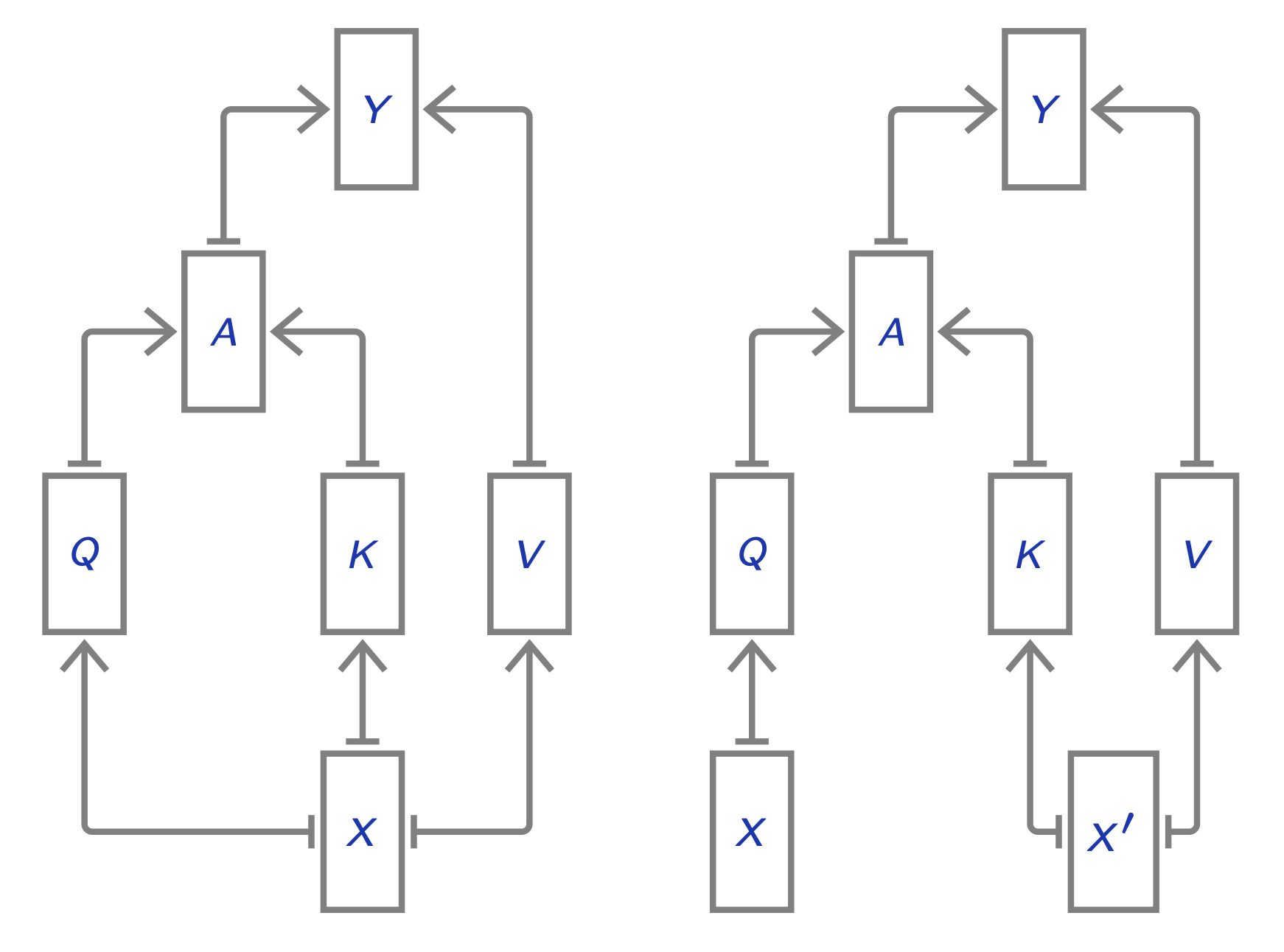
Phuong and Hutter (2022) give the following algorithm (Algorithm 4):
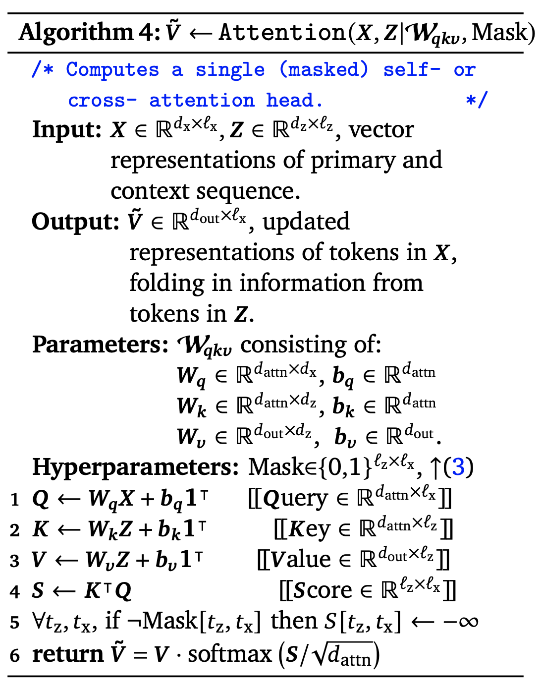
Note that there are \(\ell_{\text{X}}\) output tokens, not \(\ell_{\text{Z}}\) output tokens. This fact will be exploited in Perceiver and Perceiver IO.
Sizes of each dimension found here.
Multihead Self Attention
Split the input, run self-attention in parallel, then concatenate the output.
A popular implementation of Multi-Head attention can be found here, or by Karpathy here.
class MHSA:
  def __init__(self):
    """Initializes multi-head self attention (MHSA) layer weights."""
    ...
    # Head #1
    self.k1 = nn.Linear(self.hidden_dim, self.dim_k)
    self.v1 = nn.Linear(self.hidden_dim, self.dim_v)
    self.q1 = nn.Linear(self.hidden_dim, self.dim_q)

    # Head #2
    self.k2 = nn.Linear(self.hidden_dim, self.dim_k)
    self.v2 = nn.Linear(self.hidden_dim, self.dim_v)
    self.q2 = nn.Linear(self.hidden_dim, self.dim_q)

    self.softmax = nn.Softmax(dim=2)
    self.attention_head_projection = nn.Linear(
        self.dim_v * self.num_heads, self.hidden_dim
    )
    self.norm_mh = nn.LayerNorm(self.hidden_dim)
    ...

  def multi_head_attention(self, inputs: torch.Tensor) -> torch.Tensor:
    """Implement multi-head self-attention followed by add + norm.

    Args:
      inputs: float32 Tensor of shape (N,T,H).
      outputs: float32 Tensor of shape (N,T,H).

    Traditionally we'd include a padding mask here, so that pads are ignored.
    This is a simplified implementation.
    """
    # Based off of:
    # https://github.com/jadore801120/attention-is-all-you-need-pytorch/blob/master/transformer/SubLayers.py#L30

    batch_sz, seq_length, H = inputs.shape
    x = inputs
    identity = x

    # head 1 (project from 128-d to 96-d)
    K1 = self.k1(x)
    V1 = self.v1(x)
    Q1 = self.q1(x)

    # head 2 (project from 128-d to 96-d)
    K2 = self.k2(x)
    V2 = self.v2(x)
    Q2 = self.q2(x)

    def attention(K: torch.Tensor, Q: torch.Tensor, V: torch.Tensor, D_k: int) -> torch.Tensor:
      # within each example's sequence, get dot products of 96-d features
      # get out similarities, as (N,T,T)

      E = torch.matmul(Q, K.transpose(-2,-1)) / np.sqrt(D_k)

      A = nn.functional.softmax(E, dim=2)
      # note that A is (86,86) but V is (86,96)
      Y = torch.matmul(A, V)
      return Y

    Y1 = attention(K1, Q1, V1, D_k=self.dim_k)
    Y2 = attention(K2, Q2, V2, D_k=self.dim_k)

    # Concat to get 192-dim features
    x = torch.cat([Y1,Y2], dim=2)

    # Project back to 128d space, then apply LayerNorm.
    outputs = self.norm_mh(identity + self.attention_head_projection(x))
    return outputs
Feedforward Layer + Implementation
Every Transformer block includes a feedforward (MLP) layer. This MLP layer (with 1 hidden layer) processes each token separately. Each token is processed using the same identical weights, so it’s like a \(1 \times 1\) convolution. We can think of it as each token pondering for itself about what it has observed previously.
It contains the bulk of the parameters. When people make giant models and sparse/MoE, this is what becomes giant. GELU (Gaussian Error Linear Units) (Hendrycks et al, 2020) is used instead of ReLU.
Normalization dramatically improves trainability. In the original transformer paper, layer norm is placed on the output layer_norm(x + sublayer(x)) (post-norm) while we place layer norm on the input x + sublayer(layer_norm(x)) (pre-norm) to match GPT-2. Pre-norm has been shown to be important in improving the performance of the transformer (Xiong et al, 2020).
(See the Pytorch implementation)
import torch

class FeedforwardLayer:

  def __init__(self):
    ...
    self.linear1 = nn.Linear(self.hidden_dim, dim_feedforward)
    self.linear2 = nn.Linear(dim_feedforward, self.hidden_dim)
    self.norm1 = nn.LayerNorm(self.hidden_dim)

  def feedforward_layer(self, inputs: torch.Tensor) -> torch.Tensor:
    """Feedforward layer followed by add + norm (post-norm).

    Note that nn.Linear can operate on a tensor of any dimension, e.g. (N,...,H)

    Args:
      inputs: float32 Tensor of shape (N,T,H), where N is batch size,
        T is the sequence length, and H is the hidden dimensions.
      outputs: float32 Tensor of shape (N,T,H)
    """
    batch_sz, seq_length, H = inputs.shape
    identity = inputs
    x = inputs
    x = self.linear1(x)
    x = nn.functional.relu(x)
    x = self.linear2(x)
    x = x + identity
    x = self.norm1(x)
    outputs = x

    return outputs
Tokenization and Positional Encoding
Tokenization Input sequence is first split into pieces (Example from Lucas Beyer).
"The detective investigated" -> [The_] [detective_] [invest] [igat] [ed_]
Tokens are indices into a vocabulary.
[The_] [detective_] [invest] [igat] [ed_] -> [3 721 68 1337 42]
Each vocab entry corresponds to a learned \(d\)-dimensional vector.
[3 721 68 1337 42] -> [ [0.123, -5.234, ...], [...], [...], [...], [...] ]
Positional Encoding While attention is permutation-invariant, language (and most other tasks) are not. We need to encode the position of each word (or sequence element).
Think [The_] + 10 [detective_] + 20 [invest] + 30 … but smarter.
Enforcing Order in Self-Attention: If we permute the order of the input? Queries and Keys will be exactly the same, but permuted in order. Values will also be the same, but in different order. The outputs will also be the same, but in a different order. Thus, the self-attention layer is permutation-equivariant.
To make the processing position-aware, we would concatenate each input with a positional encoding \(E\). This encoding \(E\) helps make the function position-dependent. Note that \(E\) could simply be a learned lookup table:
def __init__(self) -> None:
    ...
    self.token_embedding_table = nn.Embedding(vocab_size, n_embd)
    self.position_embedding_table = nn.Embedding(block_size, n_embd)
    ...

def forward(self, idx: torch.Tensor, targets: torch.Tensor) -> None:
    # `idx` and `targets` are both (B,T) tensor of integers
    tok_emb = self.token_embedding_table(idx) # (B,T,C)
    pos_emb = self.position_embedding_table(torch.arange(T, device=device)) # (T,C)
    x = tok_emb + pos_emb # (B,T,C)
    ...
Above, we’ve formed our final tokens by elementwise addition of the token embedding and positional encoding.
Full Transformer and Transformer Block Definition
We’ll now describe the full Transformer architecture, which consists of stacked Transformer blocks (modules). Each module’s output has the exact same shape as its input. Following ResNets, the module computes a “residual” instead of a new value. This was shown to dramatically improve trainability.
Since input and output shapes are identical, we can stack N such blocks. Typically, N=6 (“base”), N=12 (“large”) or more.
A Transformer Block uses Self-Attention (with a residual connection), then Layer Normalization, then an MLP independently on each vector (with a residual connection), and then another Layer Norm.
A Transformer is a sequence of Transformer Blocks. To see how it is implemented, Noam Shazeer illustrates in his blog post how to do so in 27 lines of code, while still keeping clear shape hints (using the Einstein summation convention):
"""Example Transformer code with shape suffixes. [from Noam Shazeer]

Dimension key:

B: batch size
L: sequence length
M: memory length (length of sequence being attended to)
D: model dimension (sometimes called d_model or embedding_dim)
V: vocabulary size
F: feed-forward subnetwork hidden size
H: number of attention heads in a layer
K: size of each attention key or value (sometimes called d_kv)
"""

def transformer(input_token_id_BL, params):
  hidden_BLD = params.embedding_VD[input_token_id_BL]
  for layer_num in range(params.num_layers):
     hidden_BLD += attention(hiddden_BLD, params.attention_params[i])
     hidden_BLD += ffn(hiddden_BLD, params.ffn_params[i])
  hidden_BLD = layer_norm(hidden_BLD, params.final_layernorm_params)
  logits_BLV = torch.matmul(hidden_BLD, params.embedding_VD.T)
  return logits_BLV

def ffn(input_BLD, params):
   input_BLD = layer_norm(input_BLD, params.layernorm_params)
   hidden_BLF = torch.gelu(torch.matmul(input_BLD, params.w_in_DF))
   output_BLD = torch.matmul(hidden_BLF, params.w_out_FD)
   return output_BLD

def attention(input_BLD, params):
   input_BLD = layer_norm(input_BLD, params.layernorm_params)
   query_BLHK = torch.einsum('BLD,DHK->BLHK', input_BLD, params.w_q_DHK)
   key_BMHK = torch.einsum('BLD,DHK->BLHK', input_BLD, params.w_k_DHK)
   value_BMHK = torch.einsum('BLD,DHK->BLHK', input_BLD, params.w_k_DHK)
   logits_BHLM = torch.einsum('BLHK,BMHK->BHLM', query_BLHK, key_BMHK)
   B, L, H, K = query_BLHK.shape()
   logits_BHLM /= K ** 0.5
   masked_out_LM = torch.arange(L).unsqueeze(1) < torch.arange(L).unsqueeze(0)
   logits_BHLM += torch.where(masked_out_LM, -inf, 0)
   weights_BHLM = torch.softmax(logits_BHLM)
   wtd_values_BLHK = torch.einsum('BMHK,BHLM->BLHK', value_BMHK, logits_BHLM)
   out_BLD = torch.einsum('BLHK,HKD->BLD', wtd_values_BLHK, params.w_o_HKD)
   return out_BLD
Generation (Decoding)
Note that the logits may have negative values, and we need to convert them to a valid probability distribution. We feed the most recent block_size predictions back into the model as context, and keeping appending predictions to our sequence of predicted token indices.
def generate(model, idx, max_new_tokens: int):
  """idx is (B, T) array of indices in the current context."""
  for _ in range(max_new_tokens):
    # Crop idx to the last block_size tokens.
    idx_cond = idx[:, -block_size:]
    # Get the predictions
    logits, loss = model(idx_cond)
    # Focus only on the last time step.
    logits = logits[:, -1, :] # becomes (B, C)
    # Apply softmax to get probabilities.
    probs = F.softmax(logits, dim=-1) # (B, C)
    # Sample from the distribution.
    idx_next = torch.multinomial(probs, num_samples=1) # (B, 1)
    # Append sampled index to the running sequence.
    idx = torch.cat((idx, idx_next), dim=1) # (B, T+1)
    return idx
Encoder-Decoder vs. Encoder-Only vs. Decoder-Only
There are at least three important variants of the Transformer architecture today, summarized in the table below:
| Decoder-only | Encoder-only | Encoder-Decoder |
|---|---|---|
| GPT | BERT | T5 |
| Next-token prediction | Non-generative (For transfer learning), classification | generative + classification, machine translation |
| Masked MH self-attention | Non-masked MH self-attention (Cloze objective) | Masked MHSA only in decoder |
Notice that machine translation needs an Encoder-Decoder architecture, since the number of tokens differs between the input and output.
A foundational Encoder-only architecture is Bidirectional Encoder Representations from Transformer (BERT) (Devlin et al, 2018). (See Cameron Wolfe’s post).
-
Bert and T5: encoder-only or encoder-decoder with masked infill. Need many task-specific examples.
-
GPT3: decoder-only, standard left-to-right, need fewer task-specific examples.
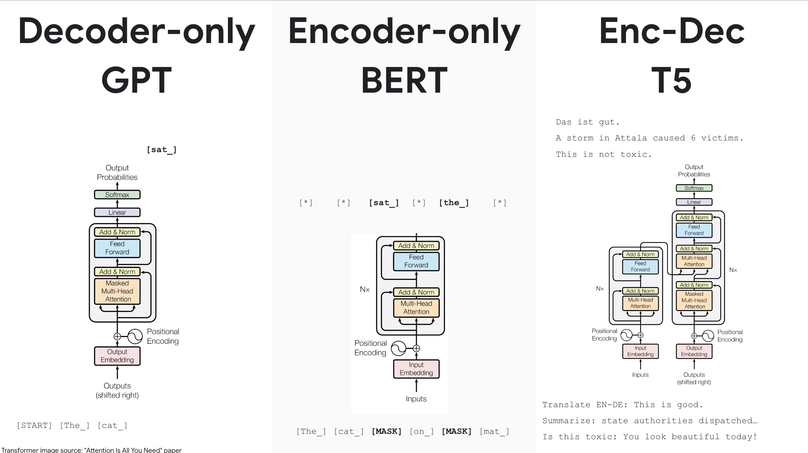
the GPT-2 architecture (Radford et al., 2019), which itself is based on the decoder of the original Transformer architecture (Vaswani et al., 2017). Perceiver’s latent Transformer (described below) also uses the GPT-2 architecture.
KV Caching for Transformers
Why not cache the queries?
What is the shape of the cache?
See gif in https://medium.com/@joaolages/kv-caching-explained-276520203249
However, there is no free lunch. The downside of KV caching is that it requires more GPU or CPU RAM.
LoRA Adapters: Low-Rank Adaptation of LLMS
Perceiver
The Perceiver architecture (Jaegle et al, 2021) builds upon the Transformer.
“an asymmetric attention mechanism to iteratively distill inputs into a tight latent bottleneck”
uses a fixed amount of latent variables, like 256 or 512. These are randomly initialized, after which they are trained end-to-end using backpropagation.
There are two key components to the Perceiver architecture:
- a cross-attention module that maps a byte array (e.g. an pixel array) and a latent array to a latent array, and
- a Transformer tower that maps a latent array to a latent array.

The size of the byte array is determined by the input data and is generally large (For an ImageNet use case, ImageNet images at resolution 224 have 50,176 pixels). The size of the latent array is a hyperparameter which is typically much smaller (e.g. the authors use 512 latents on ImageNet).
Complexity We’ll now derive the computational savings from using cross-attention with these latents. Perceiver apply attention directly to the inputs by introducing an asymmetry into the attention operation. To see how this works, first note that for \(Q \in \mathbb{R}^{M \times D}\), \(K \in \mathbb{R}^{M \times C}\) , and \(V \in \mathbb{R}^{M \times C}\) , (where \(C\) and \(D\) are channel dimensions) the complexity of the QKV attention operation – essentially, \(\mbox{softmax}(QK^T)V\) – is \(\mathcal{O}(M^2)\), as it involves two matrix multiplications with matrices of large dimension \(M\). So the authors introduce asymmetry: while \(K\) and \(V\) are projections of the input byte array, \(Q\) is a projection of a learned latent array with index dimension \(N << M\), where the latent’s index dimension \(N\) is a hyperparameter. The resulting cross-attention operation has complexity \(\mathcal{O}(MN)\).
Perceiver IO
The Perceiver IO architecture (Jaegle et al., 2021) extends the Perceiver to operate…
The main problem with the self-attention mechanism of the Transformer is that the time and memory requirements scale quadratically with the sequence length (see [Tay et al]). This is because standard self-attention compares each input to every other input at all layers.

One defines outputs of an arbitrary size, and then applies cross-attention with the last hidden states of the latents, using the outputs as queries, and the latents as keys and values.
A key part of the Perceiver are the learned latents. These can be implemented as follows (borrowing from the Hugging Face implementation) and using nn.Parameter, which allows backpropagation through them:
class PerceiverEmbeddings(nn.Module):
    """Construct the latent embeddings."""

    def __init__(self, config) -> None:
        super().__init__()
        self.latents = nn.Parameter(torch.randn(config.num_latents, config.d_latents))

    def forward(self, batch_size: int) -> torch.Tensor:
        return self.latents.expand(batch_size, -1, -1)
The Perceiver Encoder starts with cross-attention between the latents (hidden_states) and inputs:
embedding_output = self.embeddings(batch_size=batch_size)

hidden_states = embedding_output
# Inside Encoder
layer_outputs = self.cross_attention(
    hidden_states,
    attention_mask=attention_mask,
    head_mask=None,
    inputs=inputs,
    inputs_mask=inputs_mask,
    output_attentions=output_attentions,
)
hidden_states = layer_outputs[0]
Other Implementations
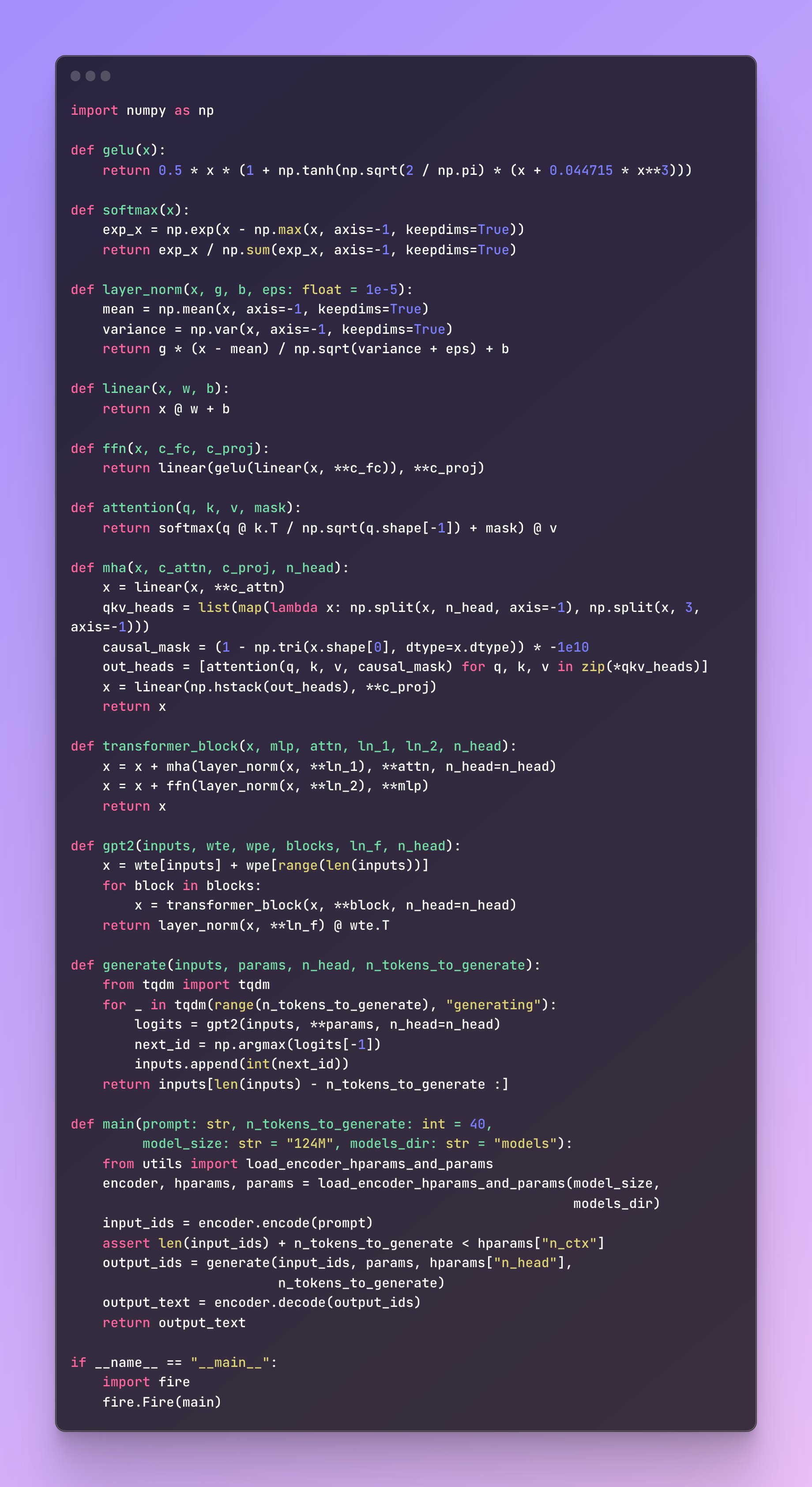
Jay Mody’s 60-line Transformer implementation in Numpy is a useful illustration of the pieces:
Vision Transformer
The Vision Transformer (ViT) (Dosovitskiy et al., 2020)…
Many prior works attempted to introduce self-attention at the pixel level. For 224px$^2$$, that’s 50k sequence length, too much!
The key breakthrough in using the full Transformer architecture, standalone, was to “tokenize” the image by cutting it into patches of 16px\(^2\), and treating each patch as a token, e.g. embedding it into input space.
Lucas Beyer: https://youtu.be/UpfcyzoZ644
Other Info
Excellent resources include The Annotated Transformer and
https://peterbloem.nl/blog/transformers
Diffusion Transformer
Diffusion Transformer (DiT) Github
import torch.nn as nn

class DiTBlock(nn.Module):
    """A DiT block with adaptive layer norm zero (adaLN-Zero) conditioning."""

    def __init__(self, hidden_size: int, num_heads: int, mlp_ratio: float = 4.0, **block_kwargs) -> None:
        """ """
        super().__init__()
        self.norm1 = nn.LayerNorm(hidden_size, elementwise_affine=False, eps=1e-6)
        self.attn = Attention(hidden_size, num_heads=num_heads, qkv_bias=True, **block_kwargs)
        self.norm2 = nn.LayerNorm(hidden_size, elementwise_affine=False, eps=1e-6)
        mlp_hidden_dim = int(hidden_size * mlp_ratio)
        approx_gelu = lambda: nn.GELU(approximate="tanh")
        self.mlp = Mlp(in_features=hidden_size, hidden_features=mlp_hidden_dim, act_layer=approx_gelu, drop=0)
        self.adaLN_modulation = nn.Sequential(
            nn.SiLU(),
            nn.Linear(hidden_size, 6 * hidden_size, bias=True)
        )

    def forward(self, x: torch.Tensor, c) -> torch.Tensor:
        shift_msa, scale_msa, gate_msa, shift_mlp, scale_mlp, gate_mlp = self.adaLN_modulation(c).chunk(6, dim=1)
        x = x + gate_msa.unsqueeze(1) * self.attn(modulate(self.norm1(x), shift_msa, scale_msa))
        x = x + gate_mlp.unsqueeze(1) * self.mlp(modulate(self.norm2(x), shift_mlp, scale_mlp))
        return x


class FinalLayer(nn.Module):
    """The final layer of DiT."""

    def __init__(self, hidden_size: int, patch_size: int, out_channels: int) -> None:
        super().__init__()
        self.norm_final = nn.LayerNorm(hidden_size, elementwise_affine=False, eps=1e-6)
        self.linear = nn.Linear(hidden_size, patch_size * patch_size * out_channels, bias=True)
        self.adaLN_modulation = nn.Sequential(
            nn.SiLU(),
            nn.Linear(hidden_size, 2 * hidden_size, bias=True)
        )

    def forward(self, x, c) -> torch.Tensor:
        shift, scale = self.adaLN_modulation(c).chunk(2, dim=1)
        x = modulate(self.norm_final(x), shift, scale)
        x = self.linear(x)
        return x


class DiT(nn.Module):
    """Diffusion model with a Transformer backbone."""

    def __init__(
        self,
        input_size: int = 32,
        patch_size: int = 2,
        in_channels: int = 4,
        hidden_size: int = 1152,
        depth: int = 28,
        num_heads: int = 16,
        mlp_ratio: float = 4.0,
        class_dropout_prob: float = 0.1,
        num_classes: int = 1000,
        learn_sigma: bool = True,
    ) -> None:
        super().__init__()
        self.learn_sigma = learn_sigma
        self.in_channels = in_channels
        self.out_channels = in_channels * 2 if learn_sigma else in_channels
        self.patch_size = patch_size
        self.num_heads = num_heads

        self.x_embedder = PatchEmbed(input_size, patch_size, in_channels, hidden_size, bias=True)
        self.t_embedder = TimestepEmbedder(hidden_size)
        self.y_embedder = LabelEmbedder(num_classes, hidden_size, class_dropout_prob)
        num_patches = self.x_embedder.num_patches
        # Will use fixed sin-cos embedding:
        self.pos_embed = nn.Parameter(torch.zeros(1, num_patches, hidden_size), requires_grad=False)

        self.blocks = nn.ModuleList([
            DiTBlock(hidden_size, num_heads, mlp_ratio=mlp_ratio) for _ in range(depth)
        ])
        self.final_layer = FinalLayer(hidden_size, patch_size, self.out_channels)
        self.initialize_weights()

    def initialize_weights(self) -> None:
        """Initialize transformer layers:"""
        def _basic_init(module):
            if isinstance(module, nn.Linear):
                torch.nn.init.xavier_uniform_(module.weight)
                if module.bias is not None:
                    nn.init.constant_(module.bias, 0)
        self.apply(_basic_init)

        # Initialize (and freeze) pos_embed by sin-cos embedding:
        pos_embed = get_2d_sincos_pos_embed(self.pos_embed.shape[-1], int(self.x_embedder.num_patches ** 0.5))
        self.pos_embed.data.copy_(torch.from_numpy(pos_embed).float().unsqueeze(0))

        # Initialize patch_embed like nn.Linear (instead of nn.Conv2d):
        w = self.x_embedder.proj.weight.data
        nn.init.xavier_uniform_(w.view([w.shape[0], -1]))
        nn.init.constant_(self.x_embedder.proj.bias, 0)

        # Initialize label embedding table:
        nn.init.normal_(self.y_embedder.embedding_table.weight, std=0.02)

        # Initialize timestep embedding MLP:
        nn.init.normal_(self.t_embedder.mlp[0].weight, std=0.02)
        nn.init.normal_(self.t_embedder.mlp[2].weight, std=0.02)

        # Zero-out adaLN modulation layers in DiT blocks:
        for block in self.blocks:
            nn.init.constant_(block.adaLN_modulation[-1].weight, 0)
            nn.init.constant_(block.adaLN_modulation[-1].bias, 0)

        # Zero-out output layers:
        nn.init.constant_(self.final_layer.adaLN_modulation[-1].weight, 0)
        nn.init.constant_(self.final_layer.adaLN_modulation[-1].bias, 0)
        nn.init.constant_(self.final_layer.linear.weight, 0)
        nn.init.constant_(self.final_layer.linear.bias, 0)

    def unpatchify(self, x: torch.Tensor) -> torch.Tensor:
        """

        Args:
            x: (N, T, patch_size**2 * C)
            imgs: (N, H, W, C)
        """
        c = self.out_channels
        p = self.x_embedder.patch_size[0]
        h = w = int(x.shape[1] ** 0.5)
        assert h * w == x.shape[1]

        x = x.reshape(shape=(x.shape[0], h, w, p, p, c))
        x = torch.einsum('nhwpqc->nchpwq', x)
        imgs = x.reshape(shape=(x.shape[0], c, h * p, h * p))
        return imgs

    def forward(self, x: torch.Tensor, t: torch.Tensor, y: torch.Tensor) -> torch.Tensor:
        """Forward pass of DiT.

        Args:
            x: (N, C, H, W) tensor of spatial inputs (images or latent representations of images)
            t: (N,) tensor of diffusion timesteps
            y: (N,) tensor of class labels
        """
        x = self.x_embedder(x) + self.pos_embed  # (N, T, D), where T = H * W / patch_size ** 2
        t = self.t_embedder(t)                   # (N, D)
        y = self.y_embedder(y, self.training)    # (N, D)
        c = t + y                                # (N, D)
        for block in self.blocks:
            x = block(x, c)                      # (N, T, D)
        x = self.final_layer(x, c)                # (N, T, patch_size ** 2 * out_channels)
        x = self.unpatchify(x)                   # (N, out_channels, H, W)
        return x
def DiT_XL_2(**kwargs):
    return DiT(depth=28, hidden_size=1152, patch_size=2, num_heads=16, **kwargs)

def DiT_XL_4(**kwargs):
    return DiT(depth=28, hidden_size=1152, patch_size=4, num_heads=16, **kwargs)

def DiT_XL_8(**kwargs):
    return DiT(depth=28, hidden_size=1152, patch_size=8, num_heads=16, **kwargs)

def DiT_L_2(**kwargs):
    return DiT(depth=24, hidden_size=1024, patch_size=2, num_heads=16, **kwargs)

def DiT_L_4(**kwargs):
    return DiT(depth=24, hidden_size=1024, patch_size=4, num_heads=16, **kwargs)

def DiT_L_8(**kwargs):
    return DiT(depth=24, hidden_size=1024, patch_size=8, num_heads=16, **kwargs)

def DiT_B_2(**kwargs):
    return DiT(depth=12, hidden_size=768, patch_size=2, num_heads=12, **kwargs)

def DiT_B_4(**kwargs):
    return DiT(depth=12, hidden_size=768, patch_size=4, num_heads=12, **kwargs)

def DiT_B_8(**kwargs):
    return DiT(depth=12, hidden_size=768, patch_size=8, num_heads=12, **kwargs)

def DiT_S_2(**kwargs):
    return DiT(depth=12, hidden_size=384, patch_size=2, num_heads=6, **kwargs)

def DiT_S_4(**kwargs):
    return DiT(depth=12, hidden_size=384, patch_size=4, num_heads=6, **kwargs)

def DiT_S_8(**kwargs):
    return DiT(depth=12, hidden_size=384, patch_size=8, num_heads=6, **kwargs)
Historical Background: Origins of QKV Attention
Now that you understand the workings of a Transformer, you may be interested in its origin story.
f query-key-value (QKV) attention (Graves et al., 2014; Weston et al., 2015; (Bahdanau et al., 2015)
Graves, A., Wayne, G., and Danihelka, I. Neural Turing machines. arXiv preprint arXiv:1410.5401, 2014.
Weston, J., Chopra, S., and Bordes, A. Memory networks. ICLR, 2015.
Bahdanau, D., Cho, K., and Bengio, Y. Neural machine translation by jointly learning to align and translate. In ICLR, 2015
Seq2Seq: Context vector captures the whole input sequence. \(s_0\) just tells the decoder how to start.
Seq2Seq with Attention
The problem above is that the input sequence is bottlenecked through fixedsized vector. So instead, we can use a new context vector at each step of decoder.
\(e_{t,i} = f_{att}(s_{t-1},h_i)\) \(e_t = softmax(a_t)\)
The new context vector at each step of the coder is computed as a linear combination of hidden states:
\[c_t = \sum\limits_i a_{t,i}h_i\]The decoder hidden state \(s_t\) at each timestep is computed as
\[s_t = g_U (y_{t-1}, s_{t-1}, c_t)\]The input sequence is no longer “bottlenecked” through a single vector.
Generalized Attention Layer
Create a vector of similarities between a single vector.
A key fact to recognize is that \(h_i\) is used above as an unordered input set \(\{ h_i \}\).
Generalizations:
- may have more than one query vector. How does each encoder hidden state \(h_t\) line up with the query \(s_t\)
- If we were to use a scaled dot product as the “Similarity function”, then we would have
- Separate key and value.
Hidden States (“Query vectors”)
External source is creating the queries \(Q\)
References
[1] Sutskever et al, “Sequence to sequence learning with neural networks”, NeurIPS 2014. [PDF].
[2] Bahdanau et al, “Neural machine translation by jointly learning to align and translate”, ICLR 2015. [PDF].
[3] Justin Johnson. “Lecture 13: Attention” Youtube. Slides (PDF).
[4] Vaswani et al. Attention Is All You Need. Neurips, 2017. [PDF].
[5] Lucas Beyer. Transformer, 2022. Slides.
[6] Andrew Jaegle, Felix Gimeno, Andrew Brock, Andrew Zisserman, Oriol Vinyals, Joao Carreira. Perceiver: General Perception with Iterative Attention. 2021. [PDF].
[7] Andrew Jaegle, Sebastian Borgeaud, Jean-Baptiste Alayrac, Carl Doersch, Catalin Ionescu, David Ding, Skanda Koppula, Daniel Zoran, Andrew Brock, Evan Shelhamer, Olivier Hénaff, Matthew M. Botvinick, Andrew Zisserman, Oriol Vinyals, Joāo Carreira. Perceiver IO: A General Architecture for Structured Inputs & Outputs. 2021. [PDF].
[8] Mary Phuong and Marcus Hutter. Formal Algorithms for Transformers. 2022. [PDF].
[9] Dmitry Kobak. Twitter. Link. Compiled into single page here and here.
[10] Alexey Dosovitskiy, Lucas Beyer, Alexander Kolesnikov, Dirk Weissenborn, Xiaohua Zhai, Thomas Unterthiner, Mostafa Dehghani, Matthias Minderer, Georg Heigold, Sylvain Gelly, Jakob Uszkoreit, Neil Houlsby. An Image is Worth 16x16 Words: Transformers for Image Recognition at Scale. 2020. [PDF]
[11] Francois Fleuret. Deep learning 13.2. Attention Mechanisms. [PDF].
[12] Ruibin Xiong, Yunchang Yang, Di He, Kai Zheng, Shuxin Zheng, Chen Xing, Huishuai Zhang, Yanyan Lan, Liwei Wang, Tie-Yan Liu. On Layer Normalization in the Transformer Architecture. 2020. [PDF].
[13] Jacob Devlin, Ming-Wei Chang, Kenton Lee, Kristina Toutanova. BERT: Pre-training of Deep Bidirectional Transformers for Language Understanding. 2018. [PDF].
[14] Edward Hu, Yelong Shen, Phillip Wallis, Zeyuan Allen-Zhu, Yuanzhi Li, Shean Wang, Lu Wang, Weizhu Chen. LoRA: Low-Rank Adaptation of Large Language Models. 2021. PDF.