Stereo and Disparity

Table of Contents:

• Stereo Vision Overview
• The Correspondence Problem
• Stereo Geometry
• Disparity
• Classical Matching Techniques
• A First Stereo Algorithm
• Disparity Map
• Cost Volumes
• Smoothing
• When is smoothing a good idea?
• Challenging Scenarios for Stereo
• MC-CNN

Stereo Vision Overview

“Stereo matching” is the task of estimating a 3D model of a scene from two or more images. The task requires finding matching pixels in the two images and converting the 2D positions of these matches into 3D depths [1]. Humans also use stereo vision, with a baseline (distance between our eyes) of 60 mm.

The basic idea is the following: a camera takes picture of the same scene, in two different positions, and we wish to recover the depth at each pixel. Depth is the missing ingredient, and the goal of computer vision here is to recover the missing depth information of the scene when and where the image was acquired. Depth is crucial for navigating in the world. It is the key to unlocking the images and using them for 3d reasoning. It allows us to understand shape of world, and what is in the image.

Keep in mind: the camera could be moving. We call 2d shifts “parallax”. If we fix the cameras’ position relative to each other, we can calibrate just once and operate under a known relationship. However, in other cases, we may need to calibrate them constantly, if cameras are constantly moving with respect to one another.

The Correspondence Problem

Think of two cameras collecting images at the same time. There are differences in the images. Notably, there will be a per pixel shift in the scene as a consequence of the camera’s new, different position in 3d space. However, if a large part of the scene is seen in both images, two pixel will correspond to the same structure (3D point) in the real world.

The correspondence problem is defined as finding a match across these two images to determine, What is the part of the scene on the right that matches that location? Previously, the community used only search techniques and optimization to solve this problem. Today, deep learning is used. The matching process is the key computation in stereo.

Stereo Geometry

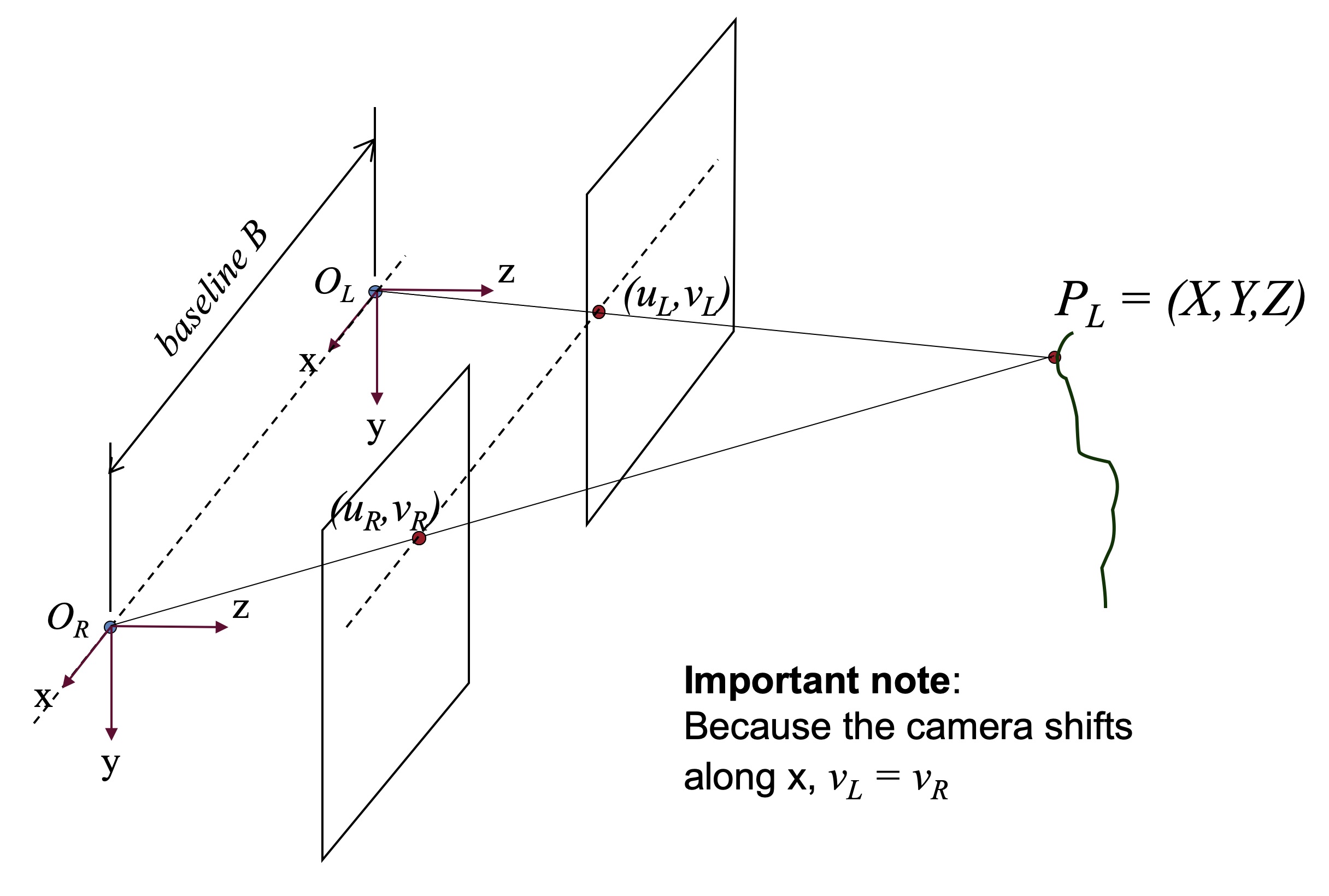
Consider the geometry of a standard, “narrow-baseline” stereo rig. If we send out two rays from a 3D scene point to the two camera centers, a triangle is constructed in the process. Our goal is to “reverse” this 3d to 2d projection.

The x-coordinate is the only difference, one is translated by the baseline $B$. shift in 1-dimension, by one number. 2 points will lie on the same row in both images. we know where to look.

there are some scale factors (which we get from calibration), simple reciprocal/inverse relationship

now, knowing geometric relationships, how to build stereo systems. Practical details: classical stereo, 80s/90s.

Consider a simple model of stereo vision: we have two cameras whose optic axes are parallel. Each camera points down the \(Z\)-axis. A figure is shown below:

Two cameras with optical centers O_L and O_R are separated by a baseline B. The z-axis extends towards the world, away from the camera.

Now, consider just the plane spanned by the \(x\)- and \(z\)-axes, with a constant \(y\) value:

Two cameras L and R are separated by a baseline b. Here the Y-axis is perpendicular to the page. f is our (horizontal) focal length.

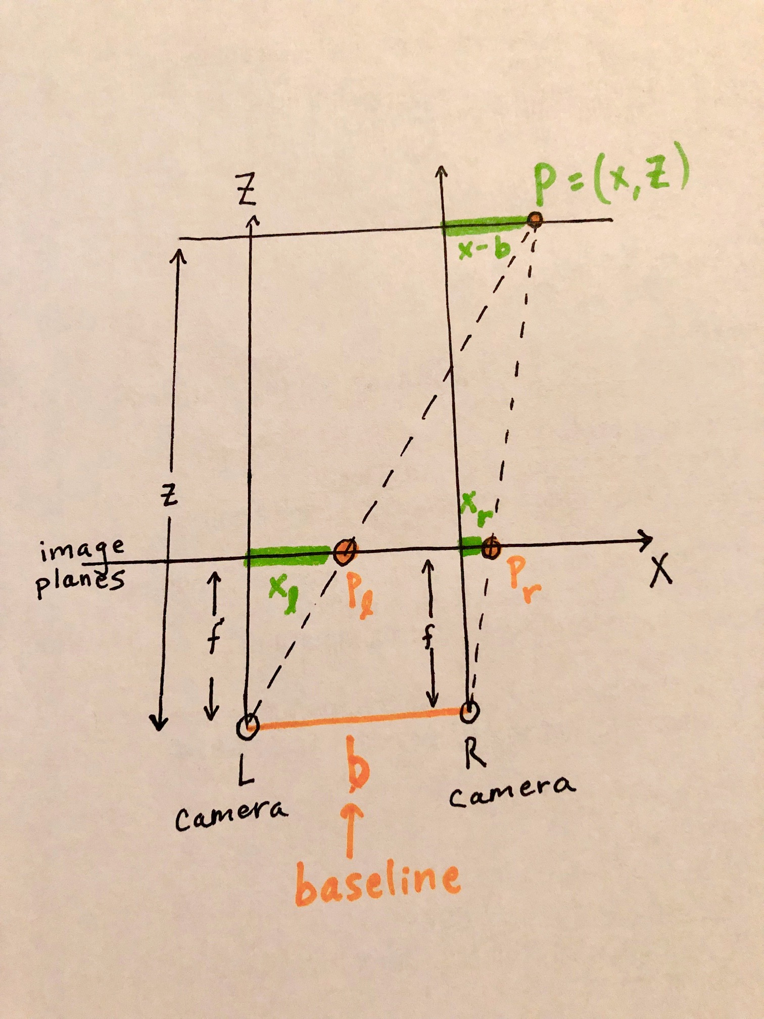
In this figure, the world point \(P=(x,z)\) is projected into the left image as \(p_l\) and into the right image as \(p_r\).

By defining right triangles we can find two similar triangles: with vertices at \((0,0)-(0,z)-(x,z)\) and \((0,0)-(0,f)-(f,x_l)\). Since they share the same angle \(\theta\), then \(\mbox{tan}(\theta)= \frac{\mbox{opposite}}{\mbox{adjacent}}\) for both, meaning:

We notice another pair of similar triangles \((b,0)-(b,z)-(x,z)\) and \((b,0)-(b,f)-(b+x_r,f)\), which by the same logic gives us

We’ll derive a closed form expression for depth in terms of disparity. We already know that

Multiply both sides by \(f\), and we get an expression for our depth from the observer:

We now want to find an expression for \(\frac{x}{x_l}\) in terms of \(x_l-x_r\), the disparity between the two images.

We can now plug this back in

Disparity

What is our takeaway? The amount of horizontal distance between the object in Image L and image R (the disparity \(d\)) is inversely proportional to the distance \(z\) from the observer. This makes perfect sense. Far away objects (large distance from the observer) will move very little between the left and right image. Very closeby objects (small distance from the observer) will move quite a bit more. The focal length \(f\) and the baseline \(b\) between the cameras are just constant scaling factors.

We made two large assumptions:

1. We know the focal length \(f\) and the baseline \(b\). This requires prior knowledge or camera calibration.
2. We need to find point correspondences, e.g. find the corresponding \((x_r,y_r)\) for each \((x_l,y_l)\).

Classical Matching Techniques

To solve the correspondence problem, we must be able to decide if two chunks of pixels (e.g. patches) are the same. How can we do so?

One classical approach is to convert the search problem into just optimizing a function. We start somewhere, and then using Newton’s Method or Gradient Descent, we can find the best match. We will place a box at every single pixel location. There will be a lot of noise in each image, so we’ll want to put a lot of measurements together to overcome that noise.

If stereo images are rectified, then all scanlines are epipolar lines. You might ask, if these epipolar lines are parallel, how do they converge? The answer is that they converge at infinity.

We’ll literally apply this formula row by row.

To convert matching to a search or optimization problem, we’ll need a vector representation and then a matching cost. Consider that an image can be thought of as a vector, if we stack each row on top of each other. Thus, a vector represents the entire image; in vector space, each point in that space is an entire image. Alternatively, each window of pixels (patch) could be a point, in which we could compare them as vectors. Inner product, or normalized correlation are measures of similarity. If we have found a good match, then the angle between the vectors will be zero, and we can use the cosine of this angle to measure this.

Two distance measures are most common for testing patch similarity, and can serve as “matching costs”:

Sum of Squared-Differences (SSD) The SSD measure is sum of squared difference of pixel values in two patches. This matching cost is measured at a proposed disparity. If \(A,B\) are patches to compare, separated by disparity \(d\), then SSD is defined as:

In this case \(A\) could be a tensor of any shape/dimensions, and \(B\) must be a tensor of the same shape as \(A\)

Sum of absolute differences (SAD) Tests if two patches are similar by the SAD distance measure. \(A,B\) are defined identically as above:

In general, absolute differences are more robust to large noise/outliers than squared differences, since outliers have less of an effect.

Search Line (Scan Line)

A correspondence will lie upon an epipolar line. Unfortunately, just because we know the Fundamental matrix betwen two images, we cannot know the exact pixel location of a match without searching for it along a 1d line (range of possible locations the pixel might appear at in the other image)

In our discussion below, we will assume that we have rectified the images, such that we can search on just a horizontal scanline.

A First Stereo Algorithm

Stereo image pair with horizontal scanline.

Given a left image, right image, similarity function, patch size, maximum search value, this algorithm will output a “disparity map”.

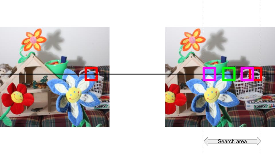
1. Pick a patch in the left image (red block), P1.
2. Place the patch in the same (x,y) coordinates in the right image (red block). As this is binocular stereo, we will need to search for P1 on the left side starting from this position. Make sure you understand this point well before proceeding further.
3. Slide the block of candidates to the left (indicated by the different pink blocks). The search area is restricted by the parameter max_search_bound in the code. The candidates will overlap.
4. We will pick the candidate patch with the minimum similarity error (green block). The horizontal shift from the red block to the green block in this image is the disparity value for the centre of P1 in the left image.

Disparity Map

Calculate the disparity value at each pixel by searching a small patch around a pixel from the left image in the right image

Note:

1. We follow the convention of search input in left image and search target in right image

2. While searching for disparity value for a patch, it may happen that there are multiple disparity values with the minimum value of the similarity measure. In that case we need to pick the smallest disparity value. Please check the numpy’s argmin and pytorch’s argmin carefully. Example: – diparity_val – | – similarity error – – 0 | 5 – 1 | 4 – 2 | 7 – 3 | 4 – 4 | 12

   In this case we need the output to be 1 and not 3.

3. The max_search_bound is defined from the patch center.

Args:

• left_img: image from the left stereo camera. Torch tensor of shape (H,W,C). C will be >= 1.
• right_img: image from the right stereo camera. Torch tensor of shape (H,W,C)
• block_size: the size of the block to be used for searching between left and right image
• sim_measure_function: a function to measure similarity measure between two tensors of the same shape; returns the error value
• max_search_bound: the maximum horizontal distance (in terms of pixels) to use for searching Returns:
• disparity_map: The map of disparity values at each pixel.

Cost Volumes

Instead of taking the argmin of the similarity error profile, one will often store the tensor of error profile at each pixel location along the third dimension.

Calculate the cost volume. Each pixel will have D=max_disparity cost values associated with it. Basically for each pixel, we compute the cost of different disparities and put them all into a tensor.

Note:

1. We’ll follow the convention of search input in left image and search target in right image
2. If the shifted patch in the right image will go out of bounds, it is good to set the default cost for that pixel and disparity to be something high(we recommend 255), so that when we consider costs, valid disparities will have a lower cost.

Args:

• left_img: image from the left stereo camera. Torch tensor of shape (H,W,C). C will be 1 or 3.
• right_img: image from the right stereo camera. Torch tensor of shape (H,W,C)
• max_disparity: represents the number of disparity values we will consider. 0 to max_disparity-1
• sim_measure_function: a function to measure similarity measure between two tensors of the same shape; returns the error value
• block_size: the size of the block to be used for searching between left and right image Returns:
• cost_volume: The cost volume tensor of shape (H,W,D). H,W are image dimensions, and D is max_disparity. cost_volume[x,y,d] represents the similarity or cost between a patch around left[x,y]
  and a patch shifted by disparity d in the right image.

Appendix B.5 and a recent survey paper on MRF inference (Szeliski, Zabih, Scharstein et al. 2008)

Error Profile

ll disparity map, we will analyse the similarity error between patches. You will have to find out different patches in the image which exhibit a close-to-convex error profile, and a highly non-convex profile.

Smoothing

One issue with the disparity maps from SSD/SAD is that they aren’t very smooth. Pixels next to each other on the same surface can have vastly different disparities, making the results look very noisy and patchy in some areas. Intuitively, pixels next to each other should have a smooth transition in disparity(unless at an object boundary or occlusion). One way to improve disparity map results is by using a smoothing constraint, such as Semi-Global Matching(SGM) or Semi-Global Block Matching. Before, we picked the disparity for a pixel based on the minimum matching cost of the block using some metric(SSD or SAD). The basic idea of SGM is to penalize pixels with a disparity that’s very different than their neighbors by adding a penalty term on top of the matching cost term.

When is smoothing a good idea?

Of course smoothing should help in noisy areas of an image. It will only help to alleviate particular types of noise, however. It is not a definitive solution to obtaining better depth maps.

Smoothing performs best on background/uniform areas: disparity values here are already similar to each other, so smoothing doesn’t have to make any drastic changes. Pixels near each other are actually supposed to have similar disparity values, so the technique makes sense in these regions. Smoothing can also help in areas of occlusion, where SAD may not be able to find any suitable match. Smoothing will curb the problems by pushing the dispairty of a pixel to be similar to that of its neighbors.

Smoothing performs poorly in areas of fine detail, with narrow objects. It also performs poorly in areas with many edges and depth discontinuities. Smoothing algorithms penalize large disparity differences in closeby regions (which can actually occur in practice). Smoothing penalizes sharp disparity changes (corresponding to depth discontinuities).

Challenges

SSD or SAD is only the beginning. SSD/SAD suffers from… large “blobs” of disparities, can have areas of large error in textureless regions. Can fail in shadows

Too small a window might not be able to distinguish unique features of an image, but too large a window would mean many patches would likely have many more things in common, leading to less helpful matches.

Note that the problem is far from solved with these approaches, as many complexities remain. Images can be problematic, and can contain areas where it is quite hard or impossible to obtain matches (e.g. under occlusion).

Consider the challenge of texture-less image regions, such as a blank wall. Here there is an issue of aggregation: one cannot look at a single white patch of pixels and tell. One must integrate info at other levels, for example by looking at the edge of wall.

Violations of the brightness constancy assumption (e.g. specular reflections) present another problem. These occur when light is reflected off of a mirror or glass picture frame, for example. Camera calibration errors would also cause problems.

What tool should we reach for to solve all of the problems in stereo?

MC-CNN

In stereo, as in almost all other computer vision tasks, convnets are the answer. However, getting deep learning into stereo took a while; for example, it took longer than recognizing cats. Our desire is for a single architecture, which will allow less propagation of error. Thus, every decision you make about how to optimize, will be end-to-end optimzation, leaving us with the best chance to drive the error down with data.

Computing the Stereo Matching Cost with a Convolutional Neural Network (MC-CNN) [9] by Zbontar and LeCun in 2015 introduced the idea of training a network to learn how to classify 2 patches as a positive vs. a negative match.

You can see how MC-CNN compares to classical approaches on the standard benchmark for stereo, which is the Middlebury Stereo Dataset and Leaderboard. At times, MC-CNN can show fine structures and succeed in shadows, when SAD and SSD cannot.

References

[1] Richard Szeliski. Computer Vision: Algorithms and Applications.

[2] James Hays. PDF.

[3] Rajesh Rao. Lecture 16: Stereo and 3D Vision, University of Washington. PDF.

[5] Yuri Boykov, Olga Veksler, Ramin Zabih. Fast Approximate Energy Minimization via Graph Cuts. ICCV 1999. PDF

[6] Zhou. Unsupervised Learning of Depth. PDF.

[7] Heiko Hirschmuller. Stereo Processing by Semi-Global Matching and Mutual Information. PDF.

[8] Heiko Hirschmuller. Semi-Global Matching – Motivation, Development, and Applications. PDF

[9] Computing the Stereo Matching Cost with a Convolutional Neural Network. Jure Zbontar and Yann LeCun. PDF.

Additional Resources: http://people.scs.carleton.ca/~c_shu/Courses/comp4900d/notes/simple_stereo.pdf http://www.cse.usf.edu/~r1k/MachineVisionBook/MachineVision.files/MachineVision_Chapter11.pdf https://courses.cs.washington.edu/courses/cse455/09wi/Lects/lect16.pdf http://cvgl.stanford.edu/teaching/cs231a_winter1415/lecture/lecture6_affine_SFM_notes.pdf https://www.cc.gatech.edu/~hays/compvision/lectures/09.pdf MRF inference (Szeliski, Zabih, Scharstein et al. 2008)