Statistical Methods

Table of Contents:

• Basic Terminology: Stats + Probability
• Discrete Distributions
• Continuous Distributions
• Generating Samples from Various Distributions: Implementation
• Central Limit Theorem (CLT)
• CLT: Visualized
• Confidence Intervals
• Computing a running mean

Basic Terminology: Statistics and Probability

In this post, I’ll discuss some basics about statistics and probability. First, we’ll define a few useful concepts:

• Population. Finite well-defined group of all objects, can be enumerated intheory (all the bearings manufactured today).

• Sample. A subset of the population (e.g. 50 out of 1000 bearings manufactured today).

• Sample is made up of observations.

• Random sample: Random variables \(X_1, X_2, \dots, X_n\) are a random sample of size \(n\) if the \(X_t\)’s are independent random variables, and every \(X_t\) has the same probability distribution.

• Probability: if we have all information about the population, we want to infer about the sample. Can be thought of as, “given the information in the pail, what is in your hand?” (Going from Population \(\rightarrow\) Sample)

• Statistics: Can be thought of as, “given the information in your hand, what is in the pail?” (Going from Sample \(\rightarrow\) Population).

• Statistical inference: make decisions about a population, based on the information contained in a random sample from that population.

• Statistic: any function of the observations in a random sample, e.g. \(X_1,X_2,\cdots,X_n \rightarrow \bar{X}, S^2\).

Discrete Distributions

Binomial

Poisson

Geometric

Negative-Binomial (Pascal)

Continuous Distributions

Exponential

Normal

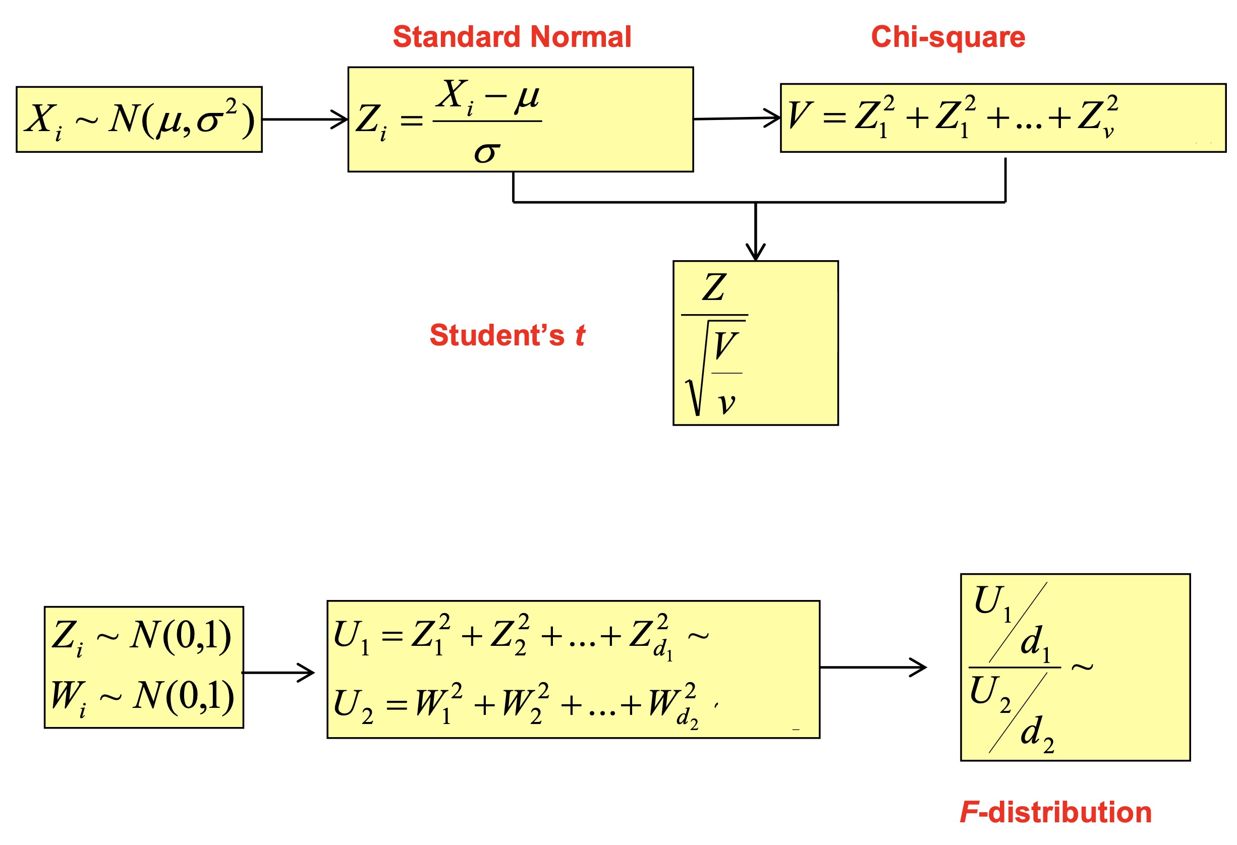
Standard Normal \(Z \sim N(0,1^2)\)

We can map any \(X\) into \(Z\): \(Z= \frac{X - \mu}{\sigma}\)

Chi-Square If \(Z_1,\dots,Z_k\) are independent, standard normal random variables, then the sum of their squares is distributed according to the chi-square distribution with \(k\) degrees of freedom.

Student’s t

Generating Samples from Various Distributions: Implementation

Plot a histogram of all 5*100 data points.

import numpy as np

x_normal = np.random.normal(loc=0.0, scale=1.0, size=(100, 5))
x_chi_sim = (x_normal ** 2).sum(axis=1)
x_chi_direct = np.random.chisquare(df=5, size=100)

import matplotlib.pyplot as plt

cum_sim = np.quantile(x_chi_sim, q=0.95)
cum_direct = np.quantile(x_chi_direct, q=0.95)
print(f"Cum. simulated vs. direct: {cum_sim} vs. {cum_direct}")

plt.subplot(1, 3, 1)
plt.hist(x_normal.squeeze(), range=[-5, 5])
plt.title("1A Normal")

plt.subplot(1, 3, 2)
plt.hist(x_chi_sim, range=[-1, 20])
plt.title("1A Chi-squared Sim.")

plt.subplot(1, 3, 3)
plt.hist(x_chi_direct, range=[-1, 20])
plt.title("1A Chi-squared Direct")
plt.show()

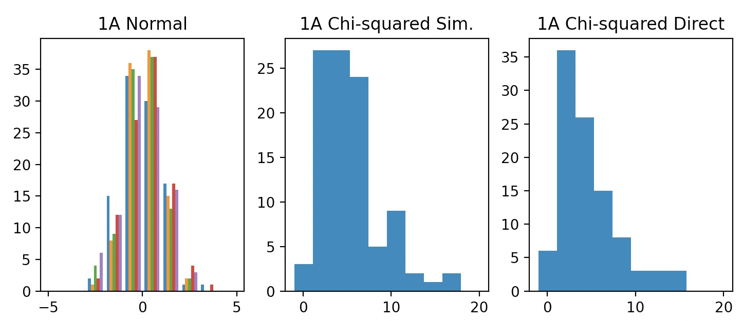
1000 samples from a standard Normal distribution \(N(0,1)\)

For each sample (row), use the definition of the Chi-squared distribution to generate one Chi-squared random number with 5 degrees of freedom. Plot the histogram for these 100 Chi-squared random numbers.

Use Python to directly generate 100 Chi-squared random numbers with 5 degrees of freedom. Plot using the histogram and compare the plots.

Find empirical \(\chi_{0.05,5}^2\) from the data using quantile as well as the exact value of qchisq function, and compare them. Note that this function works with the left tail probability.

Histogram of 5*100 Data Points

We desire to find a value of \(X=x, X \sim \chi^2(\nu)\) such that 5% of the probability mass (area under curve) lies to the right of \(X=x\) on its p.d.f. (CDF table for chi-squared measures from the right side). However, since the quantile function (similar to percentile) is measured from the left side, we use the 0.95 quantile or 95th percentile to find:\

1A. (top left) 100 samples from simulated \(\chi^2(5)\), using samples from \(N(0,1)\). (top right) 100 samples from real \(\chi^2(5)\).
Comparison: Samples from a simulated \(\chi^2(\nu)\) vs. direct \(\chi^2(\nu)\) samples look extremely similar.

Use these 100 normal random numbers and Chi-squared numbers you generated in Part a to generate 100 student’s t random numbers.

x_normal = np.random.normal(loc=0.0, scale=1.0, size=100)
x_t_direct = np.random.standard_t(df=5, size=100)
x_t_sim = x_normal / np.sqrt(x_chi_sim / 5)

cum_sim = np.quantile(x_t_sim, q=0.95)
cum_direct = np.quantile(x_t_direct, q=0.95)
print(f"Cum. simulated vs. direct: {cum_sim} vs. {cum_direct}")

plt.subplot(1, 2, 1)
plt.hist(x_t_sim, bins=20, range=[-8, 8])
plt.title("1B student t Sim.")

plt.subplot(1, 2, 2)
plt.hist(x_t_direct, bins=20, range=[-8, 8])
plt.title("1B student t Direct")
plt.show()

Cum. simulated vs. direct: 1.805 vs. 1.913

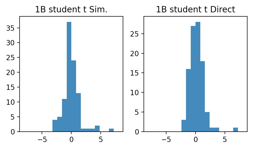
In Python, we’ll directly generate 100 \(t\) random numbers with 5 degrees of freedom, and then we’ll plot the histogram and compare the plots.

Histogram of all \(n*100\) data points:

x_chi_1df = np.random.chisquare(df=1, size=100)
x_chi_5df = np.random.chisquare(df=5, size=100)
x_F_sim = (x_chi_1df / 1) / (x_chi_5df / 5)

x_F_direct = np.random.f(dfnum=1, dfden=5, size=100)

cum_sim = np.quantile(x_F_sim, q=0.95)
cum_direct = np.quantile(x_F_direct, q=0.95)
print(f"Cum. simulated vs. direct: {cum_sim} vs. {cum_direct}")

plt.subplot(1, 2, 1)
plt.hist(x_F_sim, bins=20, range=[-1, 20])
plt.title("1C F Sim.")

plt.subplot(1, 2, 2)
plt.hist(x_F_direct, bins=20, range=[-1, 20])
plt.title("1C F Direct")
plt.show()

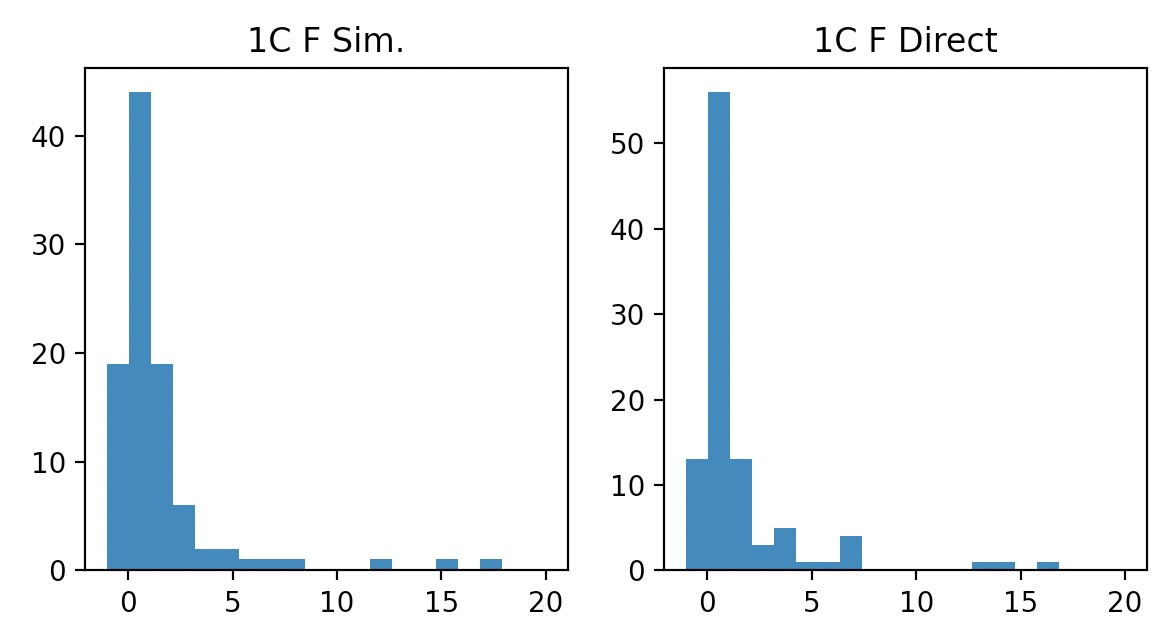
Generate one Chi-squared random number w/ 5 dof

Histogram of all n*100 data points

Central Limit Theorem (CLT)

Put simply, the CLT says that if we are sampling from a population that has an unknown probability distribution, the sampling distribution of the sample mean will still be approximately normal with mean \(\mu\) and variance \(\sigma^2/n\), if the sample size \(n\) is large.

Theorem If \(X_1,X_2,\dots, X_n\) is a random sample of size \(n\) taken from a population (Either finite or infinite) with mean \(\mu\) and finite variance \(\sigma^2\), and if \(\overline{X}\) is the sample mean, the limiting form of the distribution of \begin{equation} Z = \frac{ \overline{X}-\mu }{ \sigma / \sqrt{n} } \end{equation} as \(n \rightarrow \infty\), is the standard normal distribution.

CLT: Visualized

Suppose the underlying distribution is exponential.

We’ll compute the average of each sample (you should have 100 average values) and plot a histogram for \(\bar{X}\) values.

We’ll repeat this procedure for various n values, namely (5, 10, 30, 50, 100), and find the minimum \(n\) whose corresponding \(\bar{X}\) histogram looks normal.

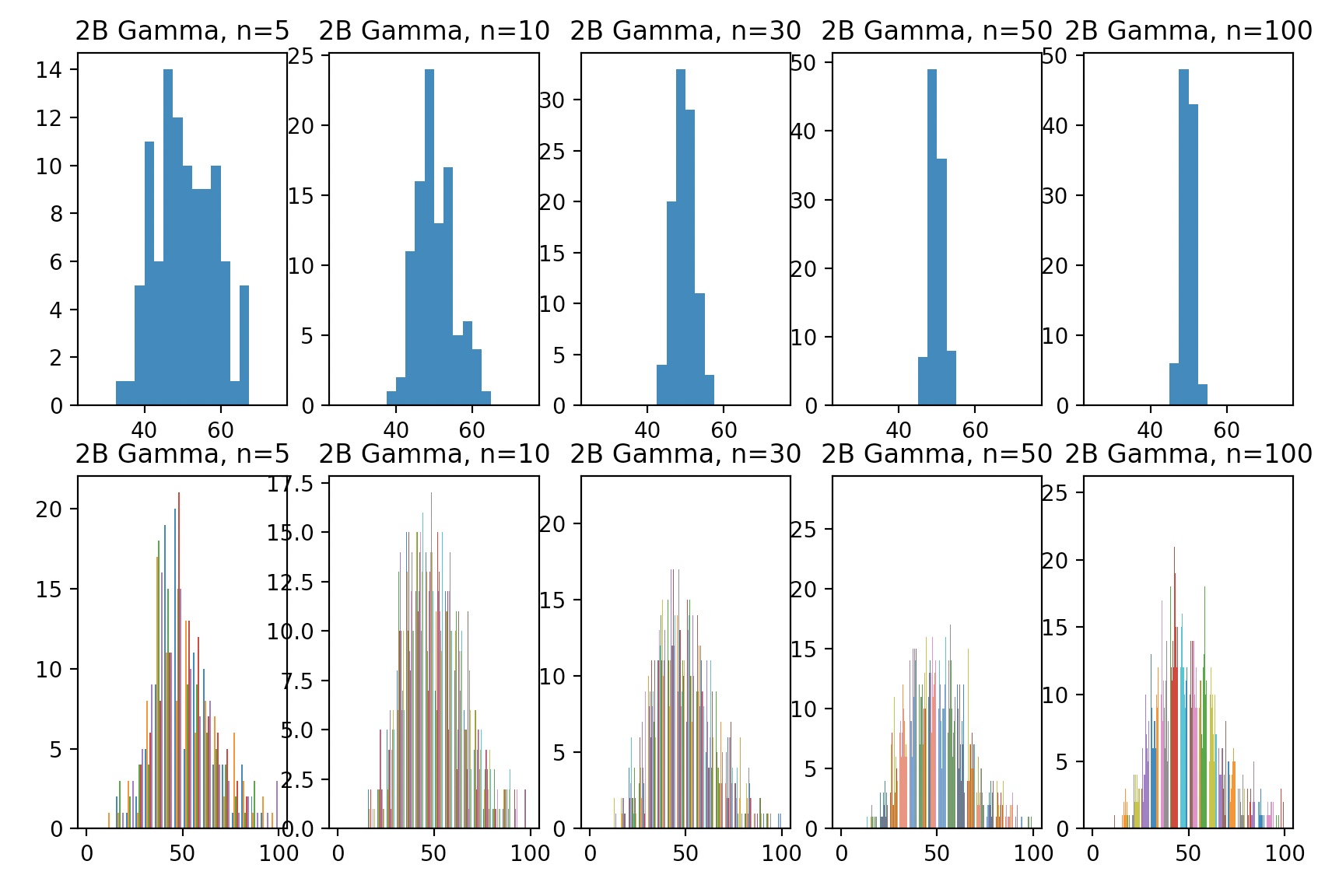
The more samples we draw and average over, the more normal the distribution looks, which follows CLT. In addition, the CLT says that your variance is inversely proportional to # samples. This is confirmed in our plots because variance is definitely shrinking as # samples grows.

exp_lambda = 0.2
n_values = [5, 10, 30, 50, 100]
for i, n in zip(range(1, 6), n_values):
    x_exp = np.random.exponential(scale=1 / exp_lambda, size=(100, n))
    x_exp_avg = np.mean(x_exp, axis=1)

    plt.subplot(2, len(n_values), i)
    plt.hist(x_exp_avg, bins=20, range=[-1, 10])
    plt.title(f"2A Exp, n={n}")

    plt.subplot(2, len(n_values), len(n_values) + i)
    plt.hist(x_exp, bins=20, range=[-1, 10])
    plt.title(f"2A Exp, n={n}")

plt.show()

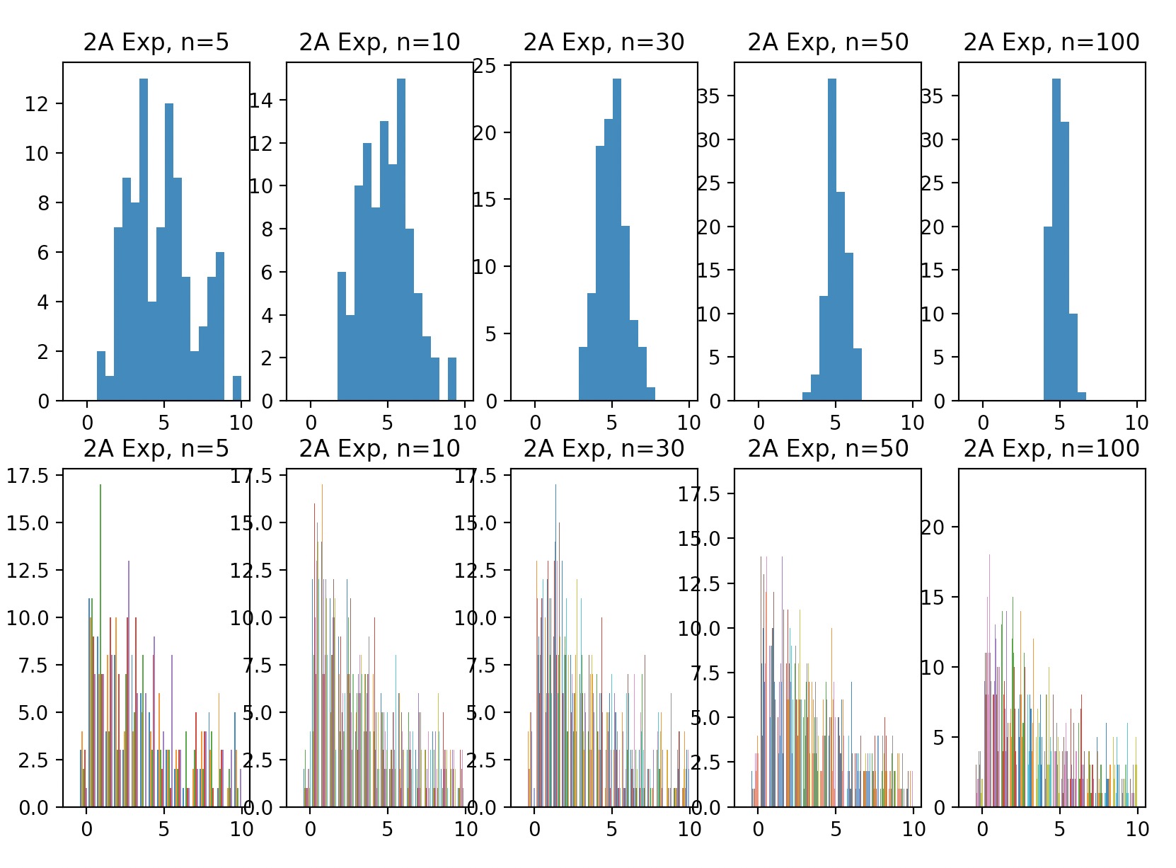
Average of each sample (100 average values), histogram of Xbar

Suppose the underlying distribution is gamma:

n_values = [5, 10, 30, 50, 100]
for i, n in zip(range(1, 6), n_values):

    x_gamma = np.random.gamma(shape=10, scale=5, size=(100, n))
    x_gamma_avg = np.mean(x_gamma, axis=1)

    plt.subplot(2, len(n_values), i)
    plt.hist(x_gamma_avg, bins=20, range=[25, 75])
    plt.title(f"2B Gamma, n={n}")

    plt.subplot(2, len(n_values), len(n_values) + i)
    plt.hist(x_gamma.squeeze(), bins=20, range=[0, 100])
    plt.title(f"2B Gamma, n={n}")

plt.show()

Confidence Intervals

Understanding the concept of confidence interval: Using Python, we’ll generate 1000 samples of 5 standard normal random numbers.

For each sample (row), find a 95% confidence interval.

We should think of this as: take 5 samples, and repeat this experiment 1000 times.

Since our samples are from \(Z \sim N(\mu=0,\sigma^2=1)\), we can compute the confidence interval as:

Percentage of intervals that cover the true mean, and conclusion

On average, how often does the population parameter of interest (here, \(\mu=0\)), belong to that interval?

We ran 3 separate random trials of our experiment.
Percentages of intervals that cover true mean, \(\mu=0\):
962 / 1000 = 96.2%,
966 / 1000 = 96.6%,
940 / 1000 = 94.0%,

Our conclusion is that (on average over several experiments), the empirical confidence interval is approximately equal to the analytical confidence interval.

simdata = np.random.randn(1000*5)
X = simdata.reshape(1000,5)
Xsums = np.sum(X,axis=1)
Xsums /= 5
np.logical_and( (Xsums + 0.877 > 0 ), (Xsums - 0.877 < 0 ) ).sum()

We also verify the percent point function (inverse of cdf – percentiles): scipy.stats.norm.ppf(0.025) = -1.96 scipy.stats.norm.ppf(0.975) = 1.96

Mean

Moments

Variance

For discrete R.V.’s:

For continuous R.V.’s:

Variance and Standard Deviation

The standard deviation is defined as the square root of the variance. The sample standard deviation is defined as:

Population variance:

One-pass Variance Computation: Welford’s Algorithm

[Add explanation of row 1]

Computing a running mean

Instead of storing a sum and a count variable, algorithm’s like Welford’s algorithm maintain a running mean with the following trick:

For a reason that will become obvious, we’ll now multiply the numerator and denominator of the left side by a constant:

We now have a very simple recurrence relation for how to update our mean \(\mu\) when a new update \(x_t\) arrives:

We must store only two variables: a count variable n, and a mean variable mu.

References

[1.]