Residual Connections in Deep Networks
Table of Contents:
- Why do we need residual connections?
- The ResNet BuildingBlock (BasicBlock)
- The ResNet Bottleneck
- Putting it all together: the full architecture
Why do we need residual connections?
An interesting phenomenon observed by many is that naively increasing network depth leads to saturated accuracy, and then rapid degradation of accuracy. The question is, why does this degradation happen?. He et al. [1] provide a convincing answer as to why, as described below.
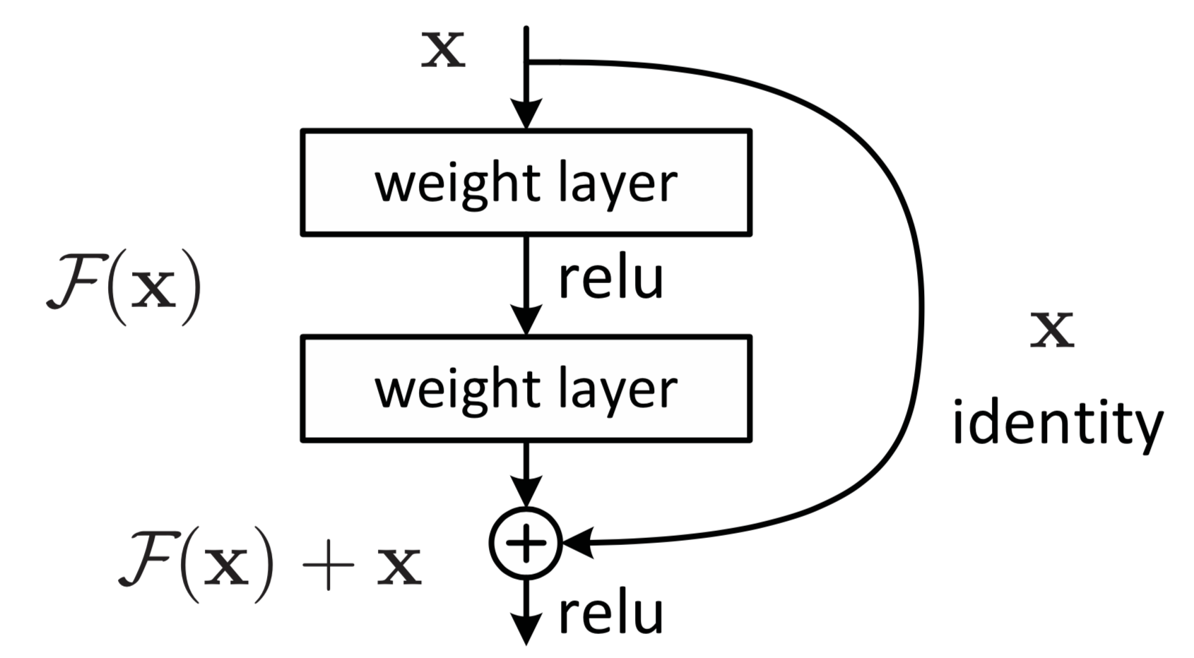
Consider a desired mapping \({\mathcal H}(x)\) we hope to achieve by stacking a few layers in a network. Instead of training these layers to fit \({\mathcal H}(x)\) directly, it may be better to train them to fit a residual mapping, i.e. \({\mathcal F}(x) := {\mathcal H}(x) − x\). The word residual means “a quantity remaining after other things have been subtracted or allowed for,” which exactly describes this relationship. We can always recover the original, desired mapping now by recasting it as:
\[{\mathcal H}(x) = {\mathcal F}(x) + x\]Why might this be better? The original mapping would be “unreferenced” – have no reference to the original input afterwards. As an extreme example, consider if an identity mapping were optimal: \({\mathcal H}(x) = x\). In this case, it is much easier to fit the residual mapping \({\mathcal F}(x)\) to return zero, then to train a stack of nonlinear layers to learn an identity mapping.
\(\begin{aligned} {\mathcal H}(x) &= {\mathcal F}(x) + x \\ x &= 0 + x \\ \end{aligned}\).
Perhaps small changes (adding a small residual) is what is optimal, and are easier to optimize. We call these connections from the input directly to the output identity shortcuts or skip-connections, and they are parameter-free. All information is always passed through them, with additional residual functions to be learned. Parameterizing \({\mathcal F}\) with weights \(W_i\), we obtain the following mapping:
\[y = {\mathcal F} (x, {W_i }) + x\]Simply put, ResNets allow for paths where information can flow more directly.
The ResNet BuildingBlock (BasicBlock)
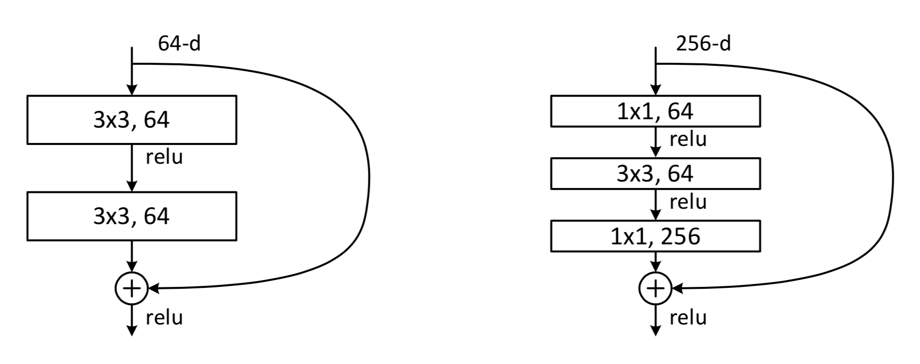
A ResNet architecture with hundreds of layers is difficult to depict. However, it is composed of just two simple, repeated modules: The BuildingBlock and the Bottleneck. I will describe the BuildingBlock here.

Consider a class that implements such a module. First we copy the input \(x\) for later, then performs two successive convolutions on the input \(x\), and then adds back the copy of \(x\), and returns the variable “\(\texttt{out}\)”. We use batch normalization after each convolution. Here is the Python code for the \(\texttt{BasicBlock}\):
class BasicBlock(nn.Module):
    expansion = 1

    def __init__(self, inplanes, planes, stride=1, downsample=None):
        super(BasicBlock, self).__init__()
        self.conv1 = conv3x3(inplanes, planes, stride)
        self.bn1 = BatchNorm(planes)
        self.relu = nn.ReLU(inplace=True)
        self.conv2 = conv3x3(planes, planes)
        self.bn2 = BatchNorm(planes)
        self.downsample = downsample
        self.stride = stride

    def forward(self, x):
        residual = x

        out = self.conv1(x)
        out = self.bn1(out)
        out = self.relu(out)

        out = self.conv2(out)
        out = self.bn2(out)

        if self.downsample is not None:
            residual = self.downsample(x)

        out += residual
        out = self.relu(out)

        return out
The ResNet Bottleneck

A slightly more complicated instantiation of the \(\texttt{BasicBlock}\) is the \(\texttt{Bottleneck}\). Instead of just two successive convolutions, the Bottleneck applies 3 successive convolutions.
class Bottleneck(nn.Module):
    expansion = 4

    def __init__(self, inplanes, planes, stride=1, downsample=None):
        super(Bottleneck, self).__init__()
        self.conv1 = nn.Conv2d(inplanes, planes, kernel_size=1, bias=False)
        self.bn1 = BatchNorm(planes)
        self.conv2 = nn.Conv2d(planes, planes, kernel_size=3, stride=stride,
                               padding=1, bias=False)
        self.bn2 = BatchNorm(planes)
        self.conv3 = nn.Conv2d(planes, planes * self.expansion, kernel_size=1, bias=False)
        self.bn3 = BatchNorm(planes * self.expansion)
        self.relu = nn.ReLU(inplace=True)
        self.downsample = downsample
        self.stride = stride

    def forward(self, x):
        residual = x

        out = self.conv1(x)
        out = self.bn1(out)
        out = self.relu(out)

        out = self.conv2(out)
        out = self.bn2(out)
        out = self.relu(out)

        out = self.conv3(out)
        out = self.bn3(out)

        if self.downsample is not None:
            residual = self.downsample(x)

        out += residual
        out = self.relu(out)

        return out
Putting it all together
There are many official variations of the ResNet architecture, with varying depth and varying performance.
Every variation has a prefix layer, four main “layers”, then an average pool, and a fully connected layer:
        self.conv1 = nn.Conv2d(3, self.inplanes, kernel_size=7, stride=2, padding=3,
                               bias=False)
        self.bn1 = norm_layer(self.inplanes)
        self.relu = nn.ReLU(inplace=True)
        self.maxpool = nn.MaxPool2d(kernel_size=3, stride=2, padding=1)
        self.layer1 = self._make_layer(block, 64, layers[0])
        self.layer2 = self._make_layer(block, 128, layers[1], stride=2,
                                       dilate=replace_stride_with_dilation[0])
        self.layer3 = self._make_layer(block, 256, layers[2], stride=2,
                                       dilate=replace_stride_with_dilation[1])
        self.layer4 = self._make_layer(block, 512, layers[3], stride=2,
                                       dilate=replace_stride_with_dilation[2])
        self.avgpool = nn.AdaptiveAvgPool2d((1, 1))
        self.fc = nn.Linear(512 * block.expansion, num_classes)
Depending upon the particular depth variation, each “layer” has a variable number of blocks.
- ResNet18: BasicBlock, [2, 2, 2, 2]
- ResNet34: BasicBlock, [3, 4, 6, 3],
- ResNet50: Bottleneck, [3, 4, 6, 3]
- ResNet101: Bottleneck, [3, 4, 23, 3]
- ResNet152: Bottleneck, [3, 8, 36, 3]
| Architecture Name | Repeated sub-module | # repetitions in Layer 0 | # repetitions in Layer 1 | # repetitions in Layer 2 | # repetitions in Layer 3 |
|---|---|---|---|---|---|
| ResNet18 | BasicBlock | 2 | 2 | 2 | 2 |
| ResNet34 | BasicBlock | 3 | 4 | 6 | 3 |
| ResNet50 | Bottleneck | 3 | 4 | 6 | 3 |
| ResNet101 | Bottleneck | 3 | 4 | 23 | 3 |
| ResNet152 | Bottleneck | 3 | 8 | 36 | 3 |
inspired by the philosophy of VGG nets. The convolutional layers mostly have 3×3 filters and follow two simple design rules:
- for the same output feature map size, the layers have the same number of filters; and
- if the feature map size is halved, the number of filters is doubled so as to preserve the time com- plexity per layer.
References
[1] Kaiming He, Xiangyu Zhang, Shaoqing Ren, Jian Sun. Deep Residual Learning for Image Recognition. CVPR 2016. PDF.
[2]. Pytorch ResNet Implementation. Github.