Linear Programming

Table of Contents:

• Weak Duality

Basic Geometric Constructs

A Convex Cone

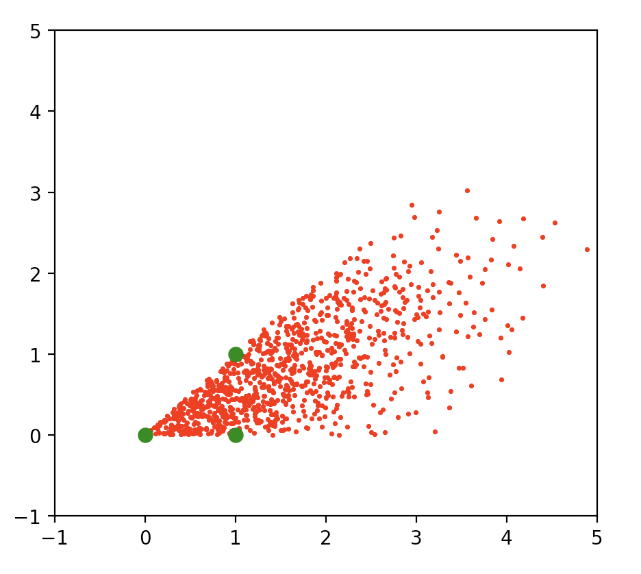
For vectors \(a_1,a_2 \in \mathbb{R}^2\), the convex cone \(\mathcal{A}\) generated by \(a_1,a_2\) is the set of weighted sums of \(a_i\) using nonnegative coefficients \(\lambda_1, \lambda_2\):

See [4,5] for more details. We’ll see an example in code, now:

import matplotlib.pyplot as plt
import numpy as np

def generate_pts_in_cone_2d(x1,x2,lambda1,lambda2)
	"""
	"""
	y = np.tile(x1,(1000,1)) * lambda1.reshape(-1,1)
	y += np.tile(x2,(1000,1)) * lambda2.reshape(-1,1)
	return y

x1 = np.array([1,0])
x2 = np.array([1,1])

lambda1 = np.absolute(np.random.randn(1000))
lambda2 = np.absolute(np.random.randn(1000))
y = generate_pts_in_cone_2d(x1,x2,lambda1,lambda2)

plt.scatter(y[:,0], y[:,1],10, c='r', marker='.')
plt.scatter(   0,      0, 200, c='g', marker='.')
plt.scatter(x1[0], x1[1], 200, c='g', marker='.')
plt.scatter(x2[0], x2[1], 200, c='g', marker='.')
plt.xlim([-1,5]); plt.ylim([-1,5]); plt.show()

More generally, the convex cone \(\mathcal{A} \in \mathbb{R}^m\) is generedated by \(n\) vectors \(a_1, a_2, \dots, a_n\).

Convex cone, anchored around the origin (0,0) and with edges passing through two other points -- (1,0) and (1,1).

Perspective: Convex Cone as a Linear System

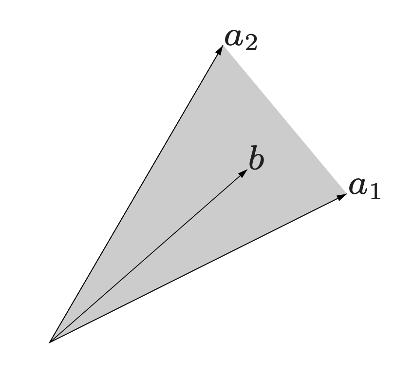
Consider the example above in \(\mathbb{R}^2\), where the two edges of our convex cone each consist of a ray extending from the origin through a point. Any point \(b\) living withiin the cone could be expressed as a weighted combinations of these two points, \(a_1, a_2\), where the weights are \(\lambda_1, \lambda_2\):

If we stack these points (each a column vector) as the columns \(a_i \in \mathbb{R}^m\) of a matrix \(A \in \mathbb{R}^{m \times n}\), we can use matrix multiplication to express the mixture of columns [1]:

where \(\lambda_1, \lambda_2\) are scalars. If instead we were to express this as \(A^T \lambda = b\), then we could have stacked the cone edge points as rows \(a_i \in \mathbb{R}^m\) of \(A \in \mathbb{R}^{n \times m}\). The coefficients of \(\lambda\) give the coefficients of mixture.

This is especially obvious when we consider \(x=e_j\), the j’th unit vector/standard basis vector:

Geometric Interpretation of Farkas’ Lemma

Farkas’ Lemma provides two possible alternatives [2]. Let \(A \in \mathbb{R}^{m \times n}\) with columns \(a_i\). We are working in m-dimensional space. In the first alternative, \(b \in \mathbb{R}^m\) lies in the cone of \(A\), which is composed of \(n\) edges.

Geometric interpretation of the first alternative. Source: [3].

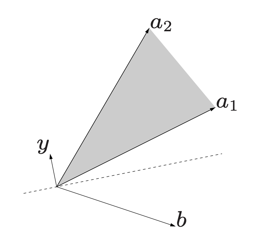
In the second alternative, there exists a hyperplane through the origin \(\mathbf{0}\), separating the vector \(b\) from the cone of \(A\). In other words, there exists a vector \(y \in \mathbb{R}^m\) such that \(y^Tb < 0\). The cone’s edge points all live on the other side of the hyperplane, such that \(y^T a_i \geq 0\). Expressed in matrix form,

In the second alternative, the angle of \(\mathbf{y}\) with the vectors \(\mathbf{a}_i\) is at most \(90^{\circ}\), while the angle of \(\mathbf {y}\) with the vector \(\mathbf{b}\) is more than \(90^{\circ}\).

The hyperplane normal to this vector has the vectors \(\mathbf{a}_i\) on one side and the vector \(\mathbf {b}\) on the other side. Hence, this hyperplane separates the vectors in the cone of \(\{\mathbf{a}_{1}, \dots ,\mathbf{a} _{n}\}\) and the vector \(\mathbf{b}\).

Geometric interpretation of the second alternative. Source: [3].

Farkas Lemma is a foundational topic. Resources from: David P. Williamson (Cornell) link, Lieven Vandenberghe on Alternatives link, Stephen Boyd on convex sets link, Ankur Moitra YouTube and transcribed notes, Michel X. Goemans link.

“If one has two systems of linear relations, where each relation is either an linear equation (or linear equality relation) or a linear inequality relation, and exactly one of the two systems has a solution, then one says that the two given systems are each others alternative.” -Kees Roos (Linear Optimization: Theorems of the Alternative).

Nonlinear Programming Cover Image Title Information Published: 1994 ISBN: 978-0-89871-341-1 eISBN: 978-1-61197-125-5 Book Code: CL10 Series: Classics in Applied Mathematics Pages: xvii + 219 Buy the Print Edition Author(s): Olvi L. Mangasarian chapter 2

Barycentric Coordinates

Farkas

https://people.orie.cornell.edu/dpw/orie6300/fall2008/Lectures/lec07.pdf

There are a few different forms for an LP. We’ll be able to use the dual to certify that our solution is optimal.

The Canonical Form

The primal problem, with solution variable \(x \in \mathbb{R}^n\). We wish to maximize a linear function. We have some constraints on what kind of \(x\) we can choose, one of which is that \(x\) is nonnegative. \(A \in \mathbb{R}^{m \times n}\), and \(\preceq\) denotes componentwise inequality:

The dual problem, with solution variable \(y\):

That is, the maximum of the primal (P) equals the minimum of the dual (D).

Weak Duality

Lemma If \(x,y\) are feasible, then \(c^Tx \leq y^Tb\).

Proof: We recall that \(x \succeq 0\), i.e. all of its entries are non-negative. Next, we recall the dual’s constraints in Canonical form, \(y^TA \succeq c^T\), which compares two column vectors with each other, at each entry. We can multiply such a column vector on the right with all non-negative scalars, and none of the inequality signs will be flipped:

Next, we recall the primal’s constraints in the Canonical form, \(Ax \preceq b\), comparing two column vectors. Since \(y\) also has all non-negative entries, we can left multiply these column vectors with \(y^T\) and not flip the sign of the inequalities:

At this point, we take a step back, flip the order of one inquality, and stack the inequalities next to each other to realize:

When combined, \(c^Tx \leq y^TAx \leq y^Tb\), as desired. \(\square\)

The Projection Theorem

Theorem: If \(\mathcal{P}\) is a non-empty closed, convex set, then:

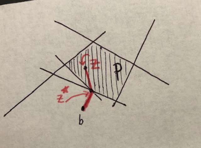
1. For any \(b\), there is a unique minimizer for \(f(z) = \| z - b \|^2\) over \(\mathcal{P}\). We call the optimal point \(z^{\star} = \mbox{proj}_{\mathcal{P}} (b)\).

2. \(z^{\star}\) is the projection of \(b\) i.f.f. \((z - z^{\star})^T (b - z) \leq 0 \hspace{7mm} \forall z \in \mathcal{P}\)

To find the closest point in a polyhedron, take a circle around \(b\), and dilate until it hits the boundary. It will hit the boundary in a unique place. If it hits the boundary in two places, then we could have undilated it slightly.

In short the vector between \((z^{\star},b)\) and the vector between \((z^{\star},z)\) could never form an acute or right angle, but rather must always form an obtuse angle. This is because \(a \cdot b = \|a\| \|b\| \mbox{cos}(\theta_{a,b})\), and unit vectors \(a,b\) with an angle \(\theta_{a,b}<90\) degrees will have dot product \(a \cdot b>0\), those with \(\theta_{a,b}=90\) degrees will have dot product of zero, and those with an obtuse angle \(\theta_{a,b}>90\) degrees will have a dot product \(a \cdot b < 0\).

Given a point b, we seek the closest point to b inside the convex set P.

The Standard Form

We will now introduce the Standard Form of LP duality, which will be useful for the Farkas’ Lemma. The primal problem, with solution variable \(x\) which must still be nonnegative:

The dual problem, with solution variable \(y\), which no longer needs to be nonnegative:

Farkas’ Lemma v1

Lemma: Exactly one of the following holds:

1. \( \exists x \mbox{ s.t. } Ax=b, \hspace{7mm} x \succeq 0\)
2. \( \exists y \mbox{ s.t. } y^TA \succeq 0 \mbox{ and } y^Tb < 0 \)

Proof: If both (1) and (2) hold, then we will show a contradiction. Let \(c=0\) in the Standard Form. We discover that \(y^Tb < c^Tx = 0\), which violates weak duality, which states that \(y^Tb\) should always be an upper bound on \(c^Tx\).

To complete the proof, we must show that when condition (1) doesn’t hold, then (2) holds. We will use the Projection Theorem to do so. Suppose there is no \(x\) that satisfies (1). We will construct \(y\) that satisfies (2).

Let \(p = \mbox{Proj}_{\mathcal{P}}(b)\), \(p=Ax\). and \(y = p-b\).

Let \(\mathcal{P}\) be a polyhedron such that \(\mathcal{P} = \{ Ax \mbox{ s.t. } x \succeq 0 \}\).

For all \(z \in \mathcal{P}\): \(\hspace{7mm} (z - p)^T(b-p) \leq 0\)

Farkas’ Lemma v2

Lemma: Exactly one of the following holds:

1. \( \exists x \mbox{ s.t. } Ax \preceq b \)

2. \( \exists y \mbox{ s.t. } y^TA = 0, \hspace{5mm} y \succeq 0, \hspace{5mm} y^Tb < 0 \)

Consider the linear system:

where \(I\) is the identity matrix, where \(x^{+}\) is the positive part of \(x\), and where \(s\) are slack variables.

Suppose we are given a solution \(x\) that satisfies \(Ax \preceq b\). Let \(x^+ = \max(x,0)\). Let \(x^- = -\min(x,0)\). Let our slack variable be defined as \(s = b - Ax\).

Farkas’ Lemma v3

Lemma: Exactly one of the following holds:

• \(y^TA \geq 0 \)
• \( b^Ty < 0 \)

Claim 1: \(y^TA \geq 0\)

Claim 2: \(b^Ty < 0\)

Strong Duality

If we take two optimal solutions to the primal and dual

References

[1] Stephen Boyd. EE 263 Course Reader PDF, Slide 2-29.

[2] Farkas’ Lemma. Wikipedia. Link.

[3] L. Vandenberghe. Lecture 5 Alternatives. PDF.

[4] Jiri Matousek Bernd Gartner. Understanding and Using Linear Programming. p. 90

[5] Stephen Boyd and Lieven Vandenberghe. Convex Optimization.