Lie Groups and Rigid Body Kinematics

Table of Contents:

• Why do we need Lie Groups?
• Lie Groups
• SO(N)
• SO(2)
• SO(3)
• SE(2)
• SE(3)
• The Lie Algebra

Why do we need Lie Groups?

Rigid bodies have a state which consists of position and orientation. When sensors are placed on a rigid body (e.g. a robot), they provide measurements in the body frame. Suppose we wish to take a measurement \(y_b\) from the body frame and move it to the world frame, yielding \(y_w\). We can do this via left multiplication with a transformation matrix \({}^{w}T_{b}\), a member of the matrix Lie groups, that transports the point from one space to another space:

What is a group?

A group is a set \(G\), with an operation \(\circ\) of (binary) multiplication on elements of \(G\) which is:

• closed: If \(g_1, g_2 \in G\) then also \(g_1 \circ g_2 \in G\);
• associative: \((g_1 \circ g_2) \circ g_3 = g_1 \circ (g_2 \circ g_3)\), for all \(g_1, g_2, g_3 \in G\);
• unit element \(e\): \(e \circ g = g \circ e = g\), for all \(g \in G\);
• invertible: For every element \(g \in G\), there exists an element \(g^{−1} \in G\) such that \(g \circ g^{−1} = g^{−1} \circ g = e\).

More details can be found in [5].

Lie Groups

When we are working with pure rotations, we work with Special Orthogonal groups, \(SO(\cdot)\). When we are working with a rotation and a translation together, we work with Special Euclidean groups \(SE(\cdot)\).

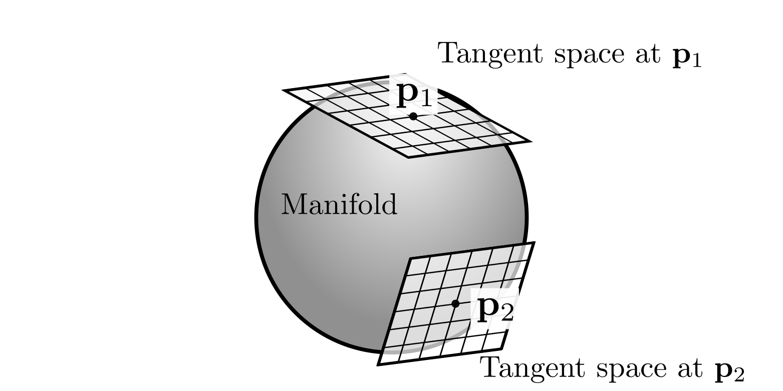
Lie Groups are unique because they are both a group and a manifold. They are continuous manifolds in high-dimensional spaces, and have a group structure. I’ll describe them in more detail below.

SO(N)

Membership in the Special Orthogonal Group \(SO(N)\) requires two matrix properties:

• \[R^TR = I\]
• \[\mbox{det}(R) = +1\]

This gives us a very helpful property: \(R^{-1} = R^T\), so the matrix inverse is as simple as taking the transpose. We will generally work with \(SO(N)\), where \(N=2,3\), meaning the matrices are rotation matrices \(R \in \mathbb{R}^{2 \times 2}\) or \(R \in \mathbb{R}^{3 \times 3}\).

These rotation matrices \(R\) are not commutative.

SO(2)

\(SO(2)\) is a 1D manifold living in a 2D Euclidean space, e.g. moving around a circle. In other words, \(SO(2)\) is the space of orthogonal matrices that corresponds to rotations in the plane. We will be stuck with singularities if we use 2 numbers to parameterize it, which would mean kinematics break down at certain orientations.

A simple example: Let’s move from the body frame \(b\) to a target frame \(t\):

As described in [3], another way to think of this is to consider that a robot can be rotated counterclockwise by some angle \(\theta \in [0,2 \pi)\) by mapping every \((x,y)\) as:

SO(3)

There are several well-known parameterizations of \(R \in SO(3)\):

1. \(R \in \mathbb{R}^{3 \times 3}\) full rotation matrix, 9 parameters – there must be 6 constraints
2. Euler angles, e.g. \((\phi, \theta, \psi)\), so 3 parameters
3. Angle-Axis parameters \((\vec{a}, \phi)\), which is 4 parameters and 1 constraint (unit length)
4. Quaternions (\(q_0,q_1,q_2,q_3)\), 4 parameters and 1 constraint (unit length)

There are only 3 degrees of freedom in describing a rotation. But this object doesn’t live in 3D space. It is a 3D manifold, embedded in a 4-D Euclidean space.

Parameterizations 1,3,4 are overconstrained, meaning they employ more parameters than we strictly need. With overparameterized representations, we have to do extra work to make sure we satisfy the constraints of the representation.

As it turns out, \(SO(3)\) cannot be parameterized by only 3 parameters in a non-singular way.

Rotation Matrices 3D rotation matrices do not form a vector space. An easy way to see this is to try to add the following two rotation matrices, \(I\) and \(R\), where \(R\) is a \(180^\circ\) rotation about the z-axis, gtsam.Rot3.RzRyRx(x=0, y=0, z=np.deg2rad(180)).matrix():

which is not a rotation (it squashes flat the x− and y− components) (See Keenan Crane’s notes here).

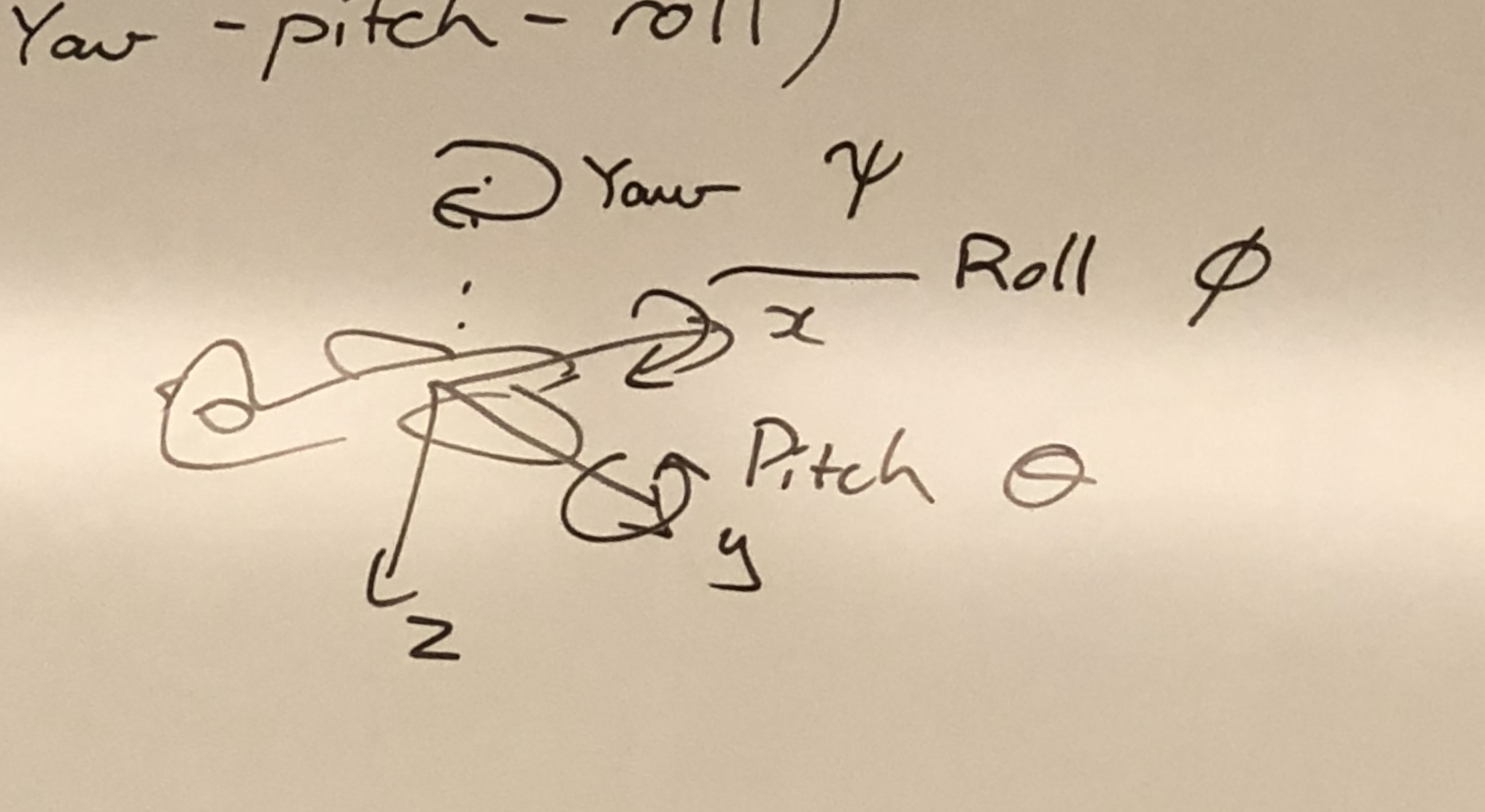
Euler Angles One parameterization of \(SO(3)\) is to imagine three successive rotations around different axes. The Euler angles encapsulate yaw-pitch-roll: first, a rotation about the x-axis by \(\phi\) (roll). Then, a rotation about the pitch axis by \(\theta\) (via right-hand rule), and finally we perform a yaw via a rotation about the z-axis (yaw, \(\psi\)).

The sequence of successive rotations is encapsulated in \({}^{w}R_b\):

As outlined in [3], these successive rotations by \((\psi, \theta, \phi)\) are defined by:

You have probably noticed that each rotation matrix \(\in \mathbb{R}^{3 \times 3}\) above is a simple extension of the 2D rotation matrix from \(SO(2)\). For example, the yaw matrix \(R_{yaw}\) performs a 2D rotation with respect to the \(x\) and \(y\) coordinates while leaving the \(z\) coordinate unchanged [3].

SE(2)

The real space \(SE(2)\) are \(3 \times 3\) matrices, moving a point in homogenous coordinates to a new frame. It is important to remember that this represents a rotation followed by a translation (not the other way around). A rigid body which translates and rotates on a 2D plane has 3 DOF, e.g. a ground robot.

By adding an extra dimension to the input points and transformation matrix \(T\), the translational part of the transformation is absorbed.

SE(3)

The set of rigid body motions, or special Euclidean transformations, is a (Lie) group, the so-called special Euclidean group, typically denoted as SE(3). The real space \(SE(3)\) is a 6-dimensional manifold. Its dimensions is exactly the number of degrees of freedom of a free-floating rigid body in space [3]. \(SE(3)\) can be parameterized with a \(4 \times 4\) matrix as follows:

What is the inverse of an SE(3) object? Consider a transformation of a point in the body frame \(p_b\) to a point in the world frame \(p_w\). Both points \(p_b, p_w\) must be in homogeneous coordinates. We can invert it as follows:

Thus if \(T = \begin{bmatrix}R & t \\ 0 & 1\end{bmatrix}\), then \(T^{-1} = \begin{bmatrix} R^T & -R^Tt \\ 0 & 1 \end{bmatrix}\). You can find my simple implementation of an object-oriented SE(3) class in Python here, or can refer to GTSAM’s Pose3 class.

Axis-Angle Representation, Lie Algebra, and Exponential and Log Maps

One of the most powerful representations of a 3d rotation is the axis-angle representation, that will allow us to compute averages of multiple rotation matrices, smoothly interpolate between two rotations, and much more. These tasks are hard to perform directly because rotation matrices don’t form a vector space—for instance, adding two rotation matrices doesn’t give you another rotation matrix [6].

We can convert rotation matrices into an axis-angle form where rotations are represented by ordinary vectors.The axis-angle representation consists of an angle \(\theta \in \mathbb{R}\) and an axis \(\mathbf{u} \in \mathbb{R}^n\). The direction of the vector gives the axis of rotation, and the magnitude of the vector gives the angle of the rotation. They define a type of “screw” motion (spinning around an axis).

We know that rotation matrices form a Lie group \(SO(n)\), and the associated vector space is the Lie algebra \(\mathfrak{so}(3)\)

• The logarithmic map can be used to turn a rotation matrix \(\mathbf{R}\) into an axis and angle.

• Manifold to tangent space: \(\mathrm{log} : SO(3) \rightarrow \mathfrak{so}(3)\)

• The exponential map can be used to turn an angle \(\theta\) and unit-length axis \(\mathbf{u}\) into a rotation matrix \(\mathbf{R}\).
• Tangent space to manifold: \(\mathrm{exp} : \mathfrak{so}(3) \rightarrow SO(3)\)

If you need to interpolate rotations across space or time, there are much better options than Euler angles. Here, rotations at the four corners are interpolated via the exp/log map. Figure source: Keenan Crane on Twitter. See CMU exercises and solutions.

The Exponential Map

The matrix exponential

defines a map from the space \(\mathfrak{so}(3)\) to \(SO(3)\), which we often call the exponential map [5].

For any rotation matrix \(R \in SO(3)\), there exists a \(\omega \in \mathbb{R}^3, \|\omega\|=1\) and \(t \in \mathbb{R}\) such that \(R = e^{ \hat{\omega}t}\). This theorem is quite powerful: it means that any rotation matrix can be realized by rotating around some fixed axis by a certain angle. This map is not one-to-one.

Exponential Map Application: Interpolation of Rotation Matrices

A problem that arises in computer vision and robotics is interpolation of rigid body motions. The following discussion is taken from Keenan Crane’s course.

We can interpolate 3d rotations using the exp/log map for 3D rotations. Given two rotations \(\mathbf{R}_0\) and \(\mathbf{R}_1\), the smallest rotation between them (in axis-angle form) is given by

Hence, we can interpolate via \(\mathbf{R}(t) = \mathrm{exp}(t \boldsymbol{\omega}) \mathbf{R}_0\).

As before, this family of rotations starts at \(t = 0\) with \(\mathbf{R}_0\), and interpolates to \(\mathbf{R}_1\) at \(t = 1\) with the minimal amount of additional “twisting” in-between.

Log / Exponential Map Application: Rotation Averaging

Another problem that arises in computer vision and robotics is single rotation averaging. The following discussion is taken from Keenan Crane’s course.

The Single Rotation Averaging problem is defined as follows: given a collection of rotation matrices \(\mathbf{R}_1, \dots, \mathbf{R}_n \in \mathbb{R}^{3 \times 3}\), find the average rotation \(\mathbf{\bar{R}}\). However, we can’t just take an average of the matrices \(\frac{1}{n} \sum\limits_{i=1}^n \mathbf{R}_i\), since the average of rotation matrices will not in general be a rotation matrix.

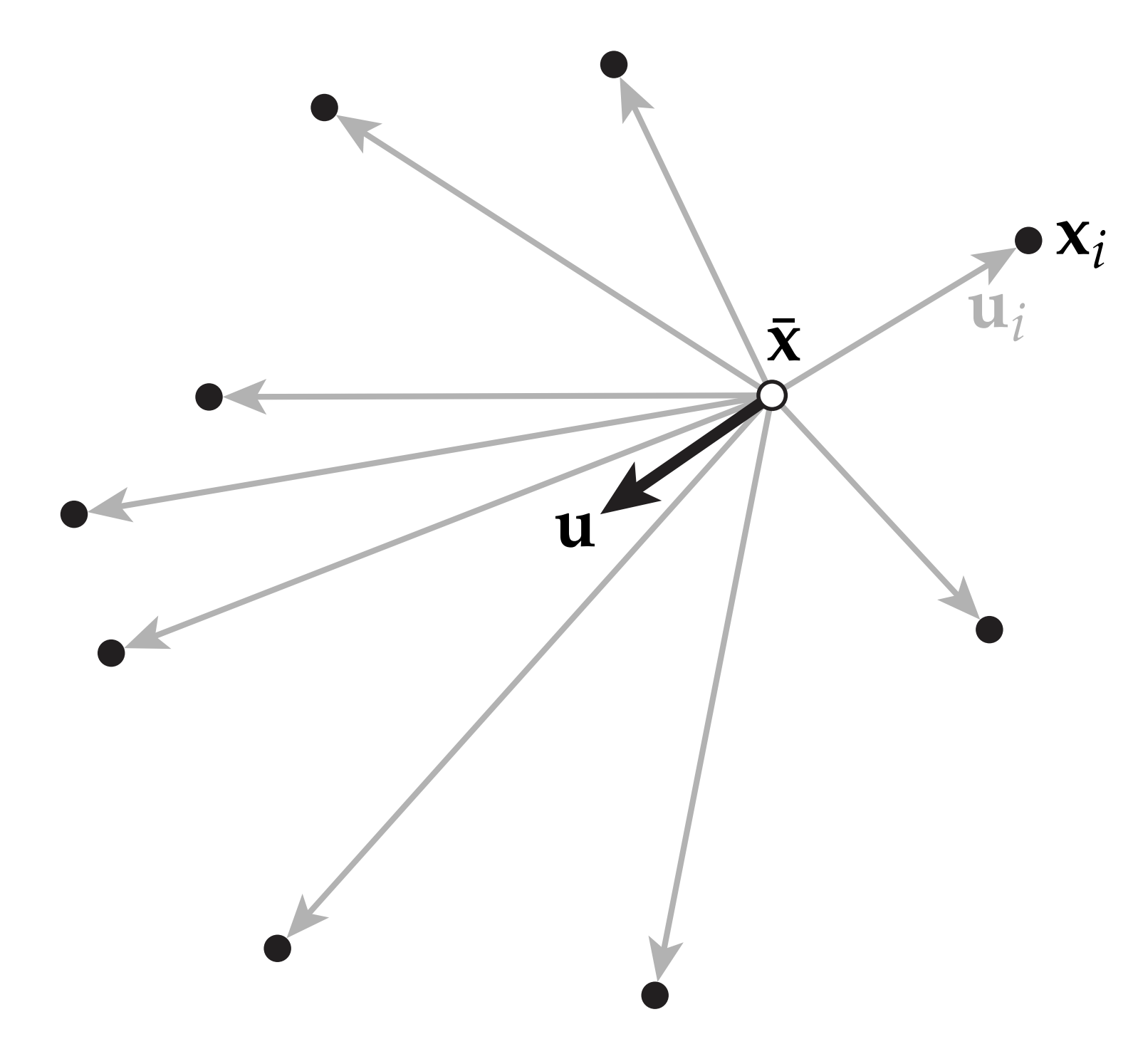
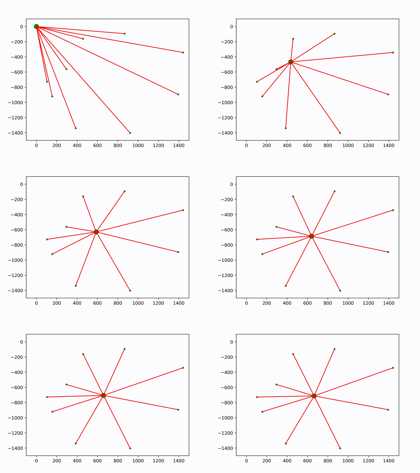
Analogy: Averaging Points. Instead, let’s first think about an unusual way to average a bunch of points \(\mathbf{x}_1, \dots, \mathbf{x}_n\) in the 2d plane. Instead of just directly taking the average (which we can’t do with rotations), we’ll pick some initial guess \(\bar{\mathbf{x}}\) for the average. We’ll then compute, for each point, the smallest vector \(\mathbf{u}_i\) that takes us from \(\mathbf{\bar{x}}\) to \(\mathbf{x}_i\). In the case of points in the 2d plane, this vector is just \(\mathbf{u}_i = \mathbf{x}_i − \mathbf{\bar{x}}\). We’ll then compute the average vector \(\mathbf{u} := \frac{1}{n} \sum\limits_{i=1}^n \mathbf{u}_i\) that tries to pull us toward all the points, and take a little step in this direction of size \(\tau \in [0, 1]\). If we reach a point where \(\mathbf{u} = 0\) – or at least, below some very small \(\epsilon > 0\)—then the algorithm stops and we know we’ve reached the average. This algorithm can be summarized as follows:

• Pick an initial guess \(\mathbf{\bar{x}} \in \mathbb{R}^2\)
• Do
  • (1) \(\mathbf{u}_i \leftarrow \mathbf{x}_i − \mathbf{\bar{x}}\)
  • (2) \(\mathbf{u} \leftarrow \frac{1}{n} \sum\limits_{i=1}^n \mathbf{u}_i\)
  • (3) \(\mathbf{\bar{x}} \leftarrow \mathbf{\bar{x}} + \tau \mathbf{u}\)
• While \(\|\mathbf{u}\| > \epsilon\)

Here are the few lines of Numpy to reproduce the iterations:

import matplotlib.pyplot as plt
import numpy as np

def compute_avg_iterative():
    """ """
    pts = np.array(
        [
            [1441, -342],
            [1393, -894],
            [921, -1403],
            [386, -1340],
            [156, -921],
            [104, -727],
            [295, -562],
            [459, -162],
            [866, -94]
        ]
    )
    tau = 0.1
    eps = 1e-3
    n = pts.shape[0]
    xbar = np.zeros(2)
    iter = 0
    while True:
        for i in range(n):
            plt.plot([xbar[0], pts[i, 0]], [xbar[1], pts[i,1]], 'r')
            plt.scatter(pts[i, 0], pts[i, 1], 10, color='g', marker='o')
        plt.scatter(xbar[0], xbar[1], 100, color='g', marker='o')
        plt.xlim([-100,1500])
        plt.ylim([-1500, 100])
        plt.savefig(f"weiszfeld_iter{iter}.jpg", dpi=400)
        plt.close("all")
        u_i = np.array([pts[i] - xbar for i in range(n)])
        u = (1/n) * np.sum(u_i, axis=0)
        xbar = xbar + tau * u
        if np.linalg.norm(u) < eps:
            break
        iter += 1

Single Rotation Averaging. The algorithm for averaging rotations is nearly identical:

• Pick an initial guess \(\mathbf{\bar{R}} \in \mathbb{R}^{3 \times 3}\)

• Do
  • (1) \(\boldsymbol{\omega}_i \leftarrow \mathrm{log}\big(\mathbf{R}_i \mathbf{\bar{R}}^{−1} \big)\)
  • (2) \(\boldsymbol{\omega}\leftarrow \frac{1}{n} \sum\limits_{i=1}^n \boldsymbol{\omega}_i\)
  • (3) \(\mathbf{\bar{R}} \leftarrow \mathrm{exp}(\tau \mbox{ } \boldsymbol{\omega})\mathbf{\bar{R}}\)
• While \(\|\boldsymbol{\omega}\| > \epsilon\)

The initial guess could be any rotation matrix—say, the identity \(\mathbf{\bar{R}} = I\). Rather than computing differences of rotation matrices, we compute the smallest rotation from \(\mathbf{\bar{R}}\) to each of the \(\mathbf{R}_i\) via the log map, yielding a bunch of skew-symmetric matrices \(\boldsymbol{\omega}_i\).

Since these matries belong to a common vector space, we can average them to produce another skew-symmetric matrix, i.e., another axis-angle representation of a rotation. Applying the exponential map moves \(\mathbf{\bar{R}}\) a little bit toward the average, and we repeat until convergence

This algorithm is essentially known as the Weiszfeld algorithm, and the notion of average we get in the end is referred to as the Karcher mean of the rotations. Multiple rotation averaging uses the same sorts of ideas, as you can see in Chatterjee and Govindu [ICCV 2013] or Shonan Averaging.

Twists

A \(4 \times 4\) matrix of the form \(\hat{\xi}\) is called a twist. The set of all twists is denoted as \(\mathfrak{se}(3)\) [4,5]:

\(\mathfrak{se}(3)\) is called the tangent space (or Lie algebra) of the matrix group \(SE(3)\).

Why do we care about twists? It turns out that a rigid body can be moved from one position to any other by a movement consisting of (1) a rotation about a straight line (2) followed by a translation parallel to that line. This type of motion is screw motion, and its infinitesimal version is called a twist. The beauty of a twist is that it describes the instantaneous velocity of a rigid body in terms of its linear and angular components, i.e. the linear velocity \(v\) and angular velocity \(\omega\)[5]. It is the matrix exponential that maps a twist into its corresponding screw motion.

References

[1] Frank Dellaert. Lecture Presentations of MM 8803: Mobile Manipulation, taught at the Georgia Institute of Technology, Fall 2018.

[2] Mac Schwager. Lecture Presentations of AA 273: State Estimation and Filtering for Aerospace Systems, taught at Stanford University in April-June 2018.

[3] Steven M. LaValle. Planning Algorithms. Cambridge University Press, 2006, New York, NY, USA. PDF.

[4] Murray, R.M., Li, Z., Sastry, S.S., Sastry, S.S.: A mathematical introduction to robotic manipulation. CRC press (1994). PDF.

[5] Ma, Yi and Soatto, Stefano and Kosecka, Jana and Sastry, S. Shankar: An Invitation to 3-D Vision: From Images to Geometric Models. Springer Verlag (2003). PDF.

[6] Keenan Crane. CMU 15-462/662. PDF.