JAX Tutorial
Table of Contents:
- JAX Intro
- JAX Arrays
- Dot Products
- Computing Gradients
- Side Effects
- JAX Training Loop: Linear Regression
- Auto-vectorization with vmap
- Optax
- Flax and Linen
- Random Number Generators in JAX
- Additional JAX Examples
JAX Intro
JAX is differentiable Numpy that runs on accelerators, and relies on a purely functional programming paradigm. We’ll discuss more about this later. It is a powerful autodifferentiation library, evolved from autograd.
The majority of this tutorial is borrowed from and gathers some of the best parts of multiple tutorials ([1],[2],[3]) to make them more accessible and self-contained. This tutorial is designed for practitioners with previous exposure to either PyTorch, Tensorflow, or Numpy.
To import JAX:
import jax
JAX Arrays The tensor analogue of np.array, tf.Tensor, and torch.Tensor is Jax’s array. We can create a vector as follows:
import jax.numpy as jnp

x = jnp.arange(10)
print(x)
# WARNING:jax._src.xla_bridge:No GPU/TPU found, falling back to CPU. (Set TF_CPP_MIN_LOG_LEVEL=0 and rerun for more info.)
# [0 1 2 3 4 5 6 7 8 9]
This same code can be run verbatim on different backends – CPU, GPU, and TPU. Unlike Numpy arrays, JAX arrays are always immutable.
Dot Products To compute a dot product of two vectors \(\in \mathbb{R}^{10^7}\) on CPU:
y = jnp.arange(int(1e7))
# Array([ 0, 1, 2, ..., 9999997, 9999998, 9999999], dtype=int32)

%timeit jnp.dot(y, y).block_until_ready()
To measure it:
CPU
# 10.6 ms ± 2.19 ms per loop (mean ± std. dev. of 7 runs, 100 loops each)
GPU
# 362 µs ± 23.6 µs per loop (mean ± std. dev. of 7 runs, 1 loop each)
Computing Gradients To compute gradients of a numerical function f written in Python, we wrap it in jax.grad, which returns a new Python function that computes the gradient of the original function f.
Consider an input array of [1,2,3,4], where the sum of its squared elements \(f(x) = \sum\limits_{i=1}^N x_i^2\) would be \(30=1+4+9+16\), and \(\nabla_x f(x) = \sum\limits_{i=1}^N 2 x_i\)
def sum_of_squares(x):
  return jnp.sum(x**2)

sum_of_squares_dx = jax.grad(sum_of_squares)
x = jnp.asarray([1., 2., 3., 4.])
print(sum_of_squares(x))
print(sum_of_squares_dx(x))
# 30.0
# [2. 4. 6. 8.]
Unlike other autodiff libraries like Tensorflow and PyTorch, in JAX, we do not compute gradients by using the loss tensor itself (e.g. by calling loss.backward() in PyTorch).
In the example above, our function \(f\) had only a single input argument, which we differentiated with respect to. We’ll now examine when we wish to compute gradients of a function that has multiple input arguments, e.g. \(f(x,y)\). By default, jax.grad() will find the gradient w.r.t. the first argument. We’ll define \(f(x,y) = \sum\limits_{i=1}^N (x_i-y_i)^2\), with \(\nabla_x f(x,y) = 2(x - y)\), and \(\nabla_y f(x,y) = -2(x-y) = 2(y-x)\)
def sum_squared_error(x, y):
  return jnp.sum((x-y)**2)

sum_squared_error_dx = jax.grad(sum_squared_error)
y = jnp.asarray([1.1, 2.1, 3.1, 4.1])
print(sum_squared_error_dx(x, y))
# [-0.20000005 -0.19999981 -0.19999981 -0.19999981]
We can compare these numerical gradients against the analytical versions:
2 * (x-y)
# Array([-0.20000005, -0.19999981, -0.19999981, -0.19999981], dtype=float32)
2 * (y-x)
# Array([0.20000005, 0.19999981, 0.19999981, 0.19999981], dtype=float32)
However, to find the error w.r.t. a different argument (or several), you can set argnums:
jax.grad(sum_squared_error, argnums=(0,1))(x,y)
# (Array([-0.20000005, -0.19999981, -0.19999981, -0.19999981], dtype=float32),
#  Array([0.20000005, 0.19999981, 0.19999981, 0.19999981], dtype=float32))
Side Effects As discussed earlier, in JAX we do not write code with side-effects. A side-effect is any effect of a function that doesn’t appear in its output. One example is modifying an array in place:
import numpy as np
x = np.array([1, 2, 3])

def in_place_modify(x):
  x[0] = 123
  return None

in_place_modify(x)
x
# array([123,   2,   3])
The side-effectful function modifies its argument, but returns a completely unrelated value.
in_place_modify(jnp.array(x))
# ---------------------------------------------------------------------------
# TypeError                                 Traceback (most recent call last)
# <ipython-input-10-930f371ec65d> in <cell line: 1>()
# ----> 1 in_place_modify(jnp.array(x))
#
# 1 frames
# /usr/local/lib/python3.9/dist-packages/jax/_src/numpy/array_methods.py in _unimplemented_setitem(self, i, x)
#     261          "or another .at[] method: "
#     262          "https://jax.readthedocs.io/en/latest/_autosummary/jax.numpy.ndarray.at.html")
# --> 263   raise TypeError(msg.format(type(self)))
#     264
#     265 def _operator_round(number: ArrayLike, ndigits: Optional[int] = None) -> Array:
#
# TypeError: '<class 'jaxlib.xla_extension.ArrayImpl'>' object does not support item assignment. JAX arrays are immutable. Instead of ``x[idx] = y``, use ``x = x.at[idx].set(y)`` or another .at[] method: https://jax.readthedocs.io/en/latest/_autosummary/jax.numpy.ndarray.at.html
Arrays can be modified in-place as follows:
import jax.numpy as jnp
x = jnp.array([5,4,3,2])
# x[1] = 10 # -> JAX arrays are immutable, so this raises a TypeError.

x = x.at[1].set(10)
print(x)  # Array[5,10,3,2], dtype=int32)
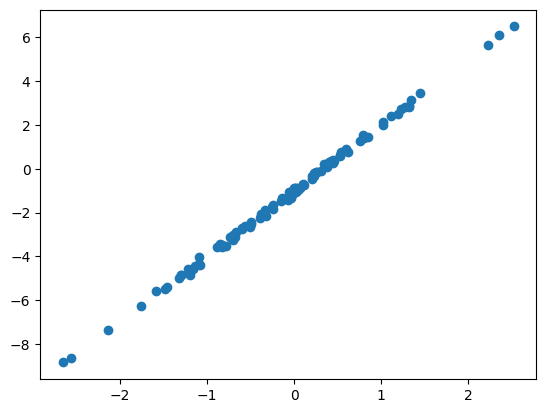
JAX Training Loop: Linear Regression We’ll implement a simple subroutine for linear regression, with data sampled as \(y = w_{true} x + b_{true} + \epsilon\)
import numpy as np
import matplotlib.pyplot as plt

xs = np.random.normal(size=(100,))
noise = np.random.normal(scale=0.1, size=(100,))
ys = xs * 3 - 1 + noise

plt.scatter(xs,ys)
Our model is \(\hat y(x; \theta) = wx + b\). We will use a single array, theta = [w, b] to house both parameters:
def model(theta, x):
  """Computes wx + b on a batch of input x."""
  w, b = theta
  return w * x + b
The loss function is \(J(x, y; \theta) = (\hat y - y)^2\):
def loss_fn(theta, x, y):
  prediction = model(theta, x)
  return jnp.mean((prediction-y)**2)
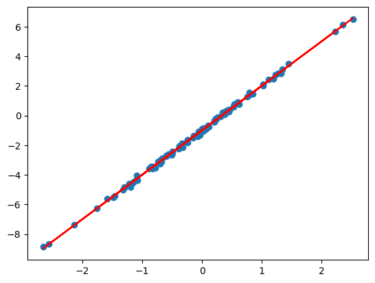
We’ll implement a simple SGD routine: \(\theta_{new} = \theta - 0.1 (\nabla_\theta J) (x, y; \theta)\)
def update(theta, x, y, lr=0.1):
  return theta - lr * jax.grad(loss_fn)(theta, x, y)
theta = jnp.array([1., 1.])

for _ in range(1000):
  theta = update(theta, xs, ys)

plt.scatter(xs, ys)
plt.plot(xs, model(theta, xs))

w, b = theta
print(f"w: {w:<.2f}, b: {b:<.2f}")
# w: 3.00, b: -1.00
Auto-vectorization with vmap
Using vmap can save you from having to carry around batch dimensions in your code.
jax.vmap
@jax.vmap
def binary_cross_entropy_with_logits(logits, labels):
  logits = nn.log_sigmoid(logits)
  return -jnp.sum(labels * logits + (1. - labels) * jnp.log(-jnp.expm1(logits)))
Optax
Optax is an optimization library that is usually used for training JAX models. It is used in a functional way, e.g.
import optax

tx = optax.adam(learning_rate=0.03)
opt_state = tx.init(variables)
updates, opt_state = tx.update(grads, opt_state)
variables = optax.apply_updates(variables, updates)
Optax includes a host of options, all the way from SGD, e.g. as tx = optax.sgd(learning_rate, momentum), to more modern variants such as AdamW and Lion.
Flax and Linen
Flax is the torch.nn equivalent of Pytorch, and the tf.keras equivalent of Tensorflow, i.e. it provides the basic neural network layers for use with JAX.
import flax
import flax.linen as nn
To get a sense for it, we’ll jump right into an example – Iimplementing an encoder/decoder for a VAE. The code will read quite similar to Pytorch VAE implementation, except much more concise! Instead of defining the network parameters in __init__(self) and forward(self), we write a single __call__(self) function in a functional style, that encapsulates all logic:
class Encoder(nn.Module):
  latents: int

  @nn.compact
  def __call__(self, x):
    x = nn.Dense(500, name='fc1')(x)
    x = nn.relu(x)
    mean_x = nn.Dense(self.latents, name='fc2_mean')(x)
    logvar_x = nn.Dense(self.latents, name='fc2_logvar')(x)
    return mean_x, logvar_x


class Decoder(nn.Module):

  @nn.compact
  def __call__(self, z):
    z = nn.Dense(500, name='fc1')(z)
    z = nn.relu(z)
    z = nn.Dense(784, name='fc2')(z)
    return z
Note the use of the function decorator nn.compact above. In Flax’s module system (named Linen), submodules and variables (parameters or others) can be defined in two ways:
- Explicitly (using
setup): Assign submodules or variables toself.<attr>inside a setup method. Then use the submodules and variables assigned toself.<attr>in setup from any “forward pass” method defined on the class. This resembles how modules are defined in PyTorch. - In-line (using
nn.compact): Write your network’s logic directly within a single “forward pass” method annotated withnn.compact. This allows you to define your whole module in a single method, and “co-locate” submodules and variables next to where they are used.
I prefer the latter, as
- Allows defining submodules, parameters and other variables next to where they are used: less scrolling up/down to see how everything is defined.
- Reduces code duplication when there are conditionals or for loops that conditionally define submodules, parameters or variables.
- Code typically looks more like mathematical notation:
y = self.param('W', ...) @ x + self.param('b', ...)looks similar to \(y=Wx+b\).
To see an example using setup instead of nn.compact,
class VAE(nn.Module):
  latents: int = 20

  def setup(self):
    self.encoder = Encoder(self.latents)
    self.decoder = Decoder()

  def __call__(self, x, z_rng):
    mean, logvar = self.encoder(x)
    z = reparameterize(z_rng, mean, logvar)
    recon_x = self.decoder(z)
    return recon_x, mean, logvar

  def generate(self, z):
    return nn.sigmoid(self.decoder(z))
Counting # of Network Parameters: An extremely useful tool of Flax is the ability to provide summaries of the number of parameters for any given network. This is encapsulated in the tabulate() method of flax.linen.Module.
As an example, consider \(28 \times 28\) pixel MNIST images, i.e. image examples \(\mathbf{x} \in \mathbb{R}^{784}\). For any batch size, and latents \(\mathbf{z} \in \mathbb{R}^{10}\), the simple encoder defined above would contained 400K params (a very small network):
encoder = Encoder(latents=10)
print(encoder.tabulate(jax.random.PRNGKey(0), jnp.ones((128, 784))))
#
#                                Encoder Summary
#┏━━━━━━━━━━━━┳━━━━━━━━━┳━━━━━━━━━━━━━━━━━━┳━━━━━━━━━━━━━━━━━━┳━━━━━━━━━━━━━━━━━┓
#┃ path       ┃ module  ┃ inputs           ┃ outputs          ┃ params          ┃
#┡━━━━━━━━━━━━╇━━━━━━━━━╇━━━━━━━━━━━━━━━━━━╇━━━━━━━━━━━━━━━━━━╇━━━━━━━━━━━━━━━━━┩
#│            │ Encoder │ float32[128,784] │ -                │                 │
#│            │         │                  │ float32[128,10]  │                 │
#│            │         │                  │ -                │                 │
#│            │         │                  │ float32[128,10]  │                 │
#├────────────┼─────────┼──────────────────┼──────────────────┼─────────────────┤
#│ fc1        │ Dense   │ float32[128,784] │ float32[128,500] │ bias:           │
#│            │         │                  │                  │ float32[500]    │
#│            │         │                  │                  │ kernel:         │
#│            │         │                  │                  │ float32[784,50… │
#│            │         │                  │                  │                 │
#│            │         │                  │                  │ 392,500 (1.6    │
#│            │         │                  │                  │ MB)             │
#├────────────┼─────────┼──────────────────┼──────────────────┼─────────────────┤
#│ fc2_mean   │ Dense   │ float32[128,500] │ float32[128,10]  │ bias:           │
#│            │         │                  │                  │ float32[10]     │
#│            │         │                  │                  │ kernel:         │
#│            │         │                  │                  │ float32[500,10] │
#│            │         │                  │                  │                 │
#│            │         │                  │                  │ 5,010 (20.0 KB) │
#├────────────┼─────────┼──────────────────┼──────────────────┼─────────────────┤
#│ fc2_logvar │ Dense   │ float32[128,500] │ float32[128,10]  │ bias:           │
#│            │         │                  │                  │ float32[10]     │
#│            │         │                  │                  │ kernel:         │
#│            │         │                  │                  │ float32[500,10] │
#│            │         │                  │                  │                 │
#│            │         │                  │                  │ 5,010 (20.0 KB) │
#├────────────┼─────────┼──────────────────┼──────────────────┼─────────────────┤
#│            │         │                  │            Total │ 402,520 (1.6    │
#│            │         │                  │                  │ MB)             │
#└────────────┴─────────┴──────────────────┴──────────────────┴─────────────────┘
#
#                       Total Parameters: 402,520 (1.6 MB)
Use of TrainState: A common pattern in Flax is to create a single dataclass that represents the entire training state, including step number, parameters, and optimizer state (flax.training.train_state.TrainState).
from flax.training import train_state

state = train_state.TrainState.create(
    apply_fn=model().apply,
    params=model().init(key, init_data, rng)['params'],
    tx=optax.adam(learning_rate),
)
Random Number Generators in JAX
The pseudo-random number generation (referred to as “PRNG”) in JAX is quite different than corresponding functionality in TensorFlow, PyTorch, or Numpy.
from jax import random

rng = random.PRNGKey(0)
rng, key = random.split(rng)

rng, z_key, eval_rng = random.split(rng, 3)

eps = random.normal(rng, logvar.shape)
Additional JAX Examples
To see high-quality examples of JAX code, you can check out the following repositories:
Equivalence with other libraries
# Create arrays
jnp.ones
jnp.zeros_like

# Create new arrays with differing shapes
jnp.stack
jnp.squeeze
jnp.concatenate

# Miscellaneous ops
jnp.exp
jnp.cumsum
jnp.mean
jnp.modf
jax.nn.one_hot
jnp.argmax
jax.random.permutation

jax.jit
nn.apply
nn.Module
nn.softplus
nn.sigmoid(raw)
num_devices = jax.local_device_count()

from flax.core import freeze, unfreeze
from flax.core.frozen_dict import FrozenDict
nn.initializers.constant(0.0),
References
-
Rosalia Schneider & Vladimir Mikulik. JAX As Accelerated NumPy. https://jax.readthedocs.io/en/latest/jax-101/01-jax-basics.html
-
Flax authors. Quickstart. https://flax.readthedocs.io/en/latest/getting_started.html
-
Flax authors. setup vs compact. https://flax.readthedocs.io/en/latest/guides/setup_or_nncompact.html