Image Derivatives and the Harris Corner Detector

Table of Contents:

• Image Derivatives
• Summed-Square Difference Error
• The Autocorrelation (AC) Surface
• Taylor Approximations of the AC Surface
• The Harris Corner Detector
• Ellipse Analogy

https://web.eecs.umich.edu/~justincj/slides/eecs442/WI2021/442_WI2021_descriptors.pdf

https://web.eecs.umich.edu/~justincj/slides/eecs442/WI2021/442_WI2021_detectors.pdf

The Autocorrelation Function

Szeliski calls this function the “auto-correlation function”, defined as:

Computationally, this is intractable. For every single patch, (for which there are width * height in the image, if we center at every possible pixel) we need compare its patch with all patches nearby it (shift_range_x * shift_range_y), and each comparison (requires patch_size_x * patch_size_y) subtraction computations.

In total, we end up with something that is

For a 600 * 600 image, with 11x11 patches, and a shift range of 11 px in both x and y, we are looking at computational complexity of: \(O(11^2 * 11^2 * 600^2) = 5.2\) billion

The auto-correlation function can alternatively be written as an error function \(E\): \(E(u,v) = \sum\limits_{x,y} w(x,y) \Bigg[ I(x+u,y+v) - I(x,y) \Bigg]^2\) where \(u\) is the shift in the \(x\) direction, \(v\) is the shift in the \(y\) direction, \(x,y\) are pixel coordinates in the image \(I\), \(w(x,y)\) is a window-ing function, and \(I(x,y)\) and \(I(x+u,y+v)\) represent intensities of pixels.

The interpretation here is to loop over all pixels in the image, and the window function will zero out everythin that is not within our window/patch of choice. The function \(E\) determines how shifting the window on \(x,y\) by some amount \(u,v\) would change the pixel values by applying the windowing function on it. This implementation is of course much less efficient, since most of the pixels in the image will not fall within the window of interest. \(E(u,v)\) indicates how much the patch intensities differ as we move the window \(w(x,y)\) a bit \((u,v)\). For the Harris Corner Detector, we want a fast rate of change for both the \(x\) and \(y\) direction over a small shift to be a corner. Thus, it measurea a changes in appearance of the window.

Deriving an Efficient Approximation

Consider a first order approximation of the image function \(I_0(\mathbf{x}_i + \Delta \mathbf{u}) \approx I_0(\mathbf{x}_i) + \nabla I_0(\mathbf{x}_i) \cdot \Delta \mathbf{u}\). Expanding terms, we will find a quadratic in \(\Delta \mathbf{u}\):

We now have a quadratic function. The auto-correlation/second-moment matrix is also known as the “structure tensor”.

Image Derivatives

    ksize = 7
    sigma = 5

    g = cv2.getGaussianKernel(ksize=ksize, sigma=sigma)
    small_filter = g * g.T

    if grad_approx_method == 'np_grad':
        ky, kx = np.gradient(filter)

    elif grad_approx_method == 'finite_diff':
        kx = np.zeros(filter.shape)
        ky = np.zeros(filter.shape)
        kx[:, :-1] = np.diff(filter, n=1, axis=1) # compute gradient on x-direction
        ky[:-1, :] = np.diff(filter, n=1, axis=0) # compute gradient on y-direction

    elif grad_approx_method == 'cv2_sobel':
        kx = cv2.Sobel(filter, cv2.CV_64F, 1, 0, ksize=3) / 8.
        ky = cv2.Sobel(filter, cv2.CV_64F, 0, 1, ksize=3) / 8.

    elif grad_approx_method == 'scipy_sobel':
        sobel_x = np.array([[1, 0, -1],
                            [2, 0, -2],
                            [1, 0, -1]])
        sobel_y = np.array([[1, 2, 1],
                            [0, 0, 0],
                            [-1, -2, -1]])
        kx = scipy.signal.convolve2d(  in1 = filter,
                                        in2 = sobel_x,
                                        mode = 'same',
                                        boundary = 'fill',
                                        fillvalue = 0) / 8.
        ky = scipy.signal.convolve2d(  in1 = filter,
                                        in2 = sobel_y,
                                        mode = 'same',
                                        boundary = 'fill',
                                        fillvalue = 0) / 8.
    return kx,ky

Image Derivatives

Great question – there are a number of ways to do it, and they will all give different results.

Convolving (not cross-correlation filtering) with the Sobel filter is a good way to approximate image derivatives (here we could treat a Gaussian filter as the image to find its derivatives).

We’ve recommended a number of potentially useful OpenCV and SciPy functions that can do so in the project page. These will be very helpful!

Another simple way to approximate the derivative is to calculate the 1st discrete difference along the given axis. For example, in order to compute horizontal discrete differences, shift the image by 1 pixel to the left and subtract the two

For example, suppose you have a matrix b

b = np.array([[ 0, 1, 1, 2],

   [  3,   5,   8,  13],

   [ 21,  34,  55,  89],

   [144, 233, 377, 610]])

b[:,1:] - b[:,:-1] We would get:

array([[ 1, 0, 1],

   [  2,   3,   5],

   [ 13,  21,  34],

   [ 89, 144, 233]])

Then we could the pad the matrix with zeros on the right column to bring it back to the original size.

Sobel vs. Gaussian

Hi, I’m trying to decide which is a better way to compute the gradient for the Harris corner detection, before I compute my cornerness function. I’m confused about the difference between both.

If I run just Sobel on my image, that means I’m getting the derivative, and smoothing with Gaussian in one go, right? And if I want to use Gaussian, I find the derivatives of the pixels, and apply Gaussian separately on the image? Not sure if one way is better than the other, and why.

You can also do both with one filter.

Suppose we have the image \(I\):

One way to think about the Sobel x-derivative filter is that rather than looking at only \(\frac{rise}{run}=\frac{f-d}{2}\) (centered at pixel e), we also use the x-derivatives above it and below it, e.g. \(\frac{c-a}{2}\) and \(\frac{i-g}{2}\). But we weight the x-derivative in the center the most (this is a form of smoothing) so we use an approximation like

meaning our kernel resembles

It is actually derived with directional derivatives. https://www.researchgate.net/publication/239398674_An_Isotropic_3_3_Image_Gradient_Operator

This is not identical to first blurring the image with a Gaussian filter, and then computing derivatives. We blur the image first because it makes the gradients less noisy.

https://d1b10bmlvqabco.cloudfront.net/attach/jl1qtqdkuye2rp/jl1r1s4npvog2/jm1ficspl6jw/smoothing_gradients.png

https://d1b10bmlvqabco.cloudfront.net/attach/jl1qtqdkuye2rp/jl1r1s4npvog2/jm1fiqeigs2g/derivative_theorem.png

And an elegant fact that can save a step in smoothed gradient computation is to simply blur with the x and y derivatives of a Gaussian filter, by the following property:

http://vision.stanford.edu/teaching/cs131_fall1617/lectures/lecture5_edges_cs131_2016.pdf Slides

The Autocorrelation Function/Surface

Suppose we wish to match a keypoint in image \(I_0\) with a keypoint in an image \(I_1\). Matching RGB values at a single pixel location will be completely uninformative. However, comparing local patches around the supposed keypoints can be quite effective because the local window captures necessary context.

Suppose we shift image \(I_1\) by displacement \(\mathbf{u} = (u,v)\), and then compare its shifted RGB values with \(I_0\). This function of weighted summed square difference (WSSD) error is known as the autocorrelation function or surface [1]. We compute the values of this function at every single possible displacement \(\mathbf{u}\). We loop over \(i\) locations in the local window neighborhood and at each \(x_i = (x,y)\), compute the difference:

This is accomplished in a few lines of Python (code here):

window_h = patch_img.shape[0]
window_w = patch_img.shape[1]

img_h = mtn_img.shape[0]
img_w = mtn_img.shape[1]

e_ssd = np.zeros((img_h-window_h,img_w-window_w))

# start at top-left corner
for u in range(0,img_h-window_h,5):
	for v in range(0,img_w-window_w,5):
		e_ssd[u,v] = np.square(mtn_img[u:u+window_h:,v:v+window_w,:] - patch_img).sum()

Left: Original mountain scene from [1]. Right: Centered patch cropped from the image.

Left: 3D surface plot of the error function. Blue is lower error, red is higher error. Center: Overhead (bird's eye view) of the 3D surface plot. Right: The localized patch, computed using the displacement that minimizes the error function, is plotted in red.

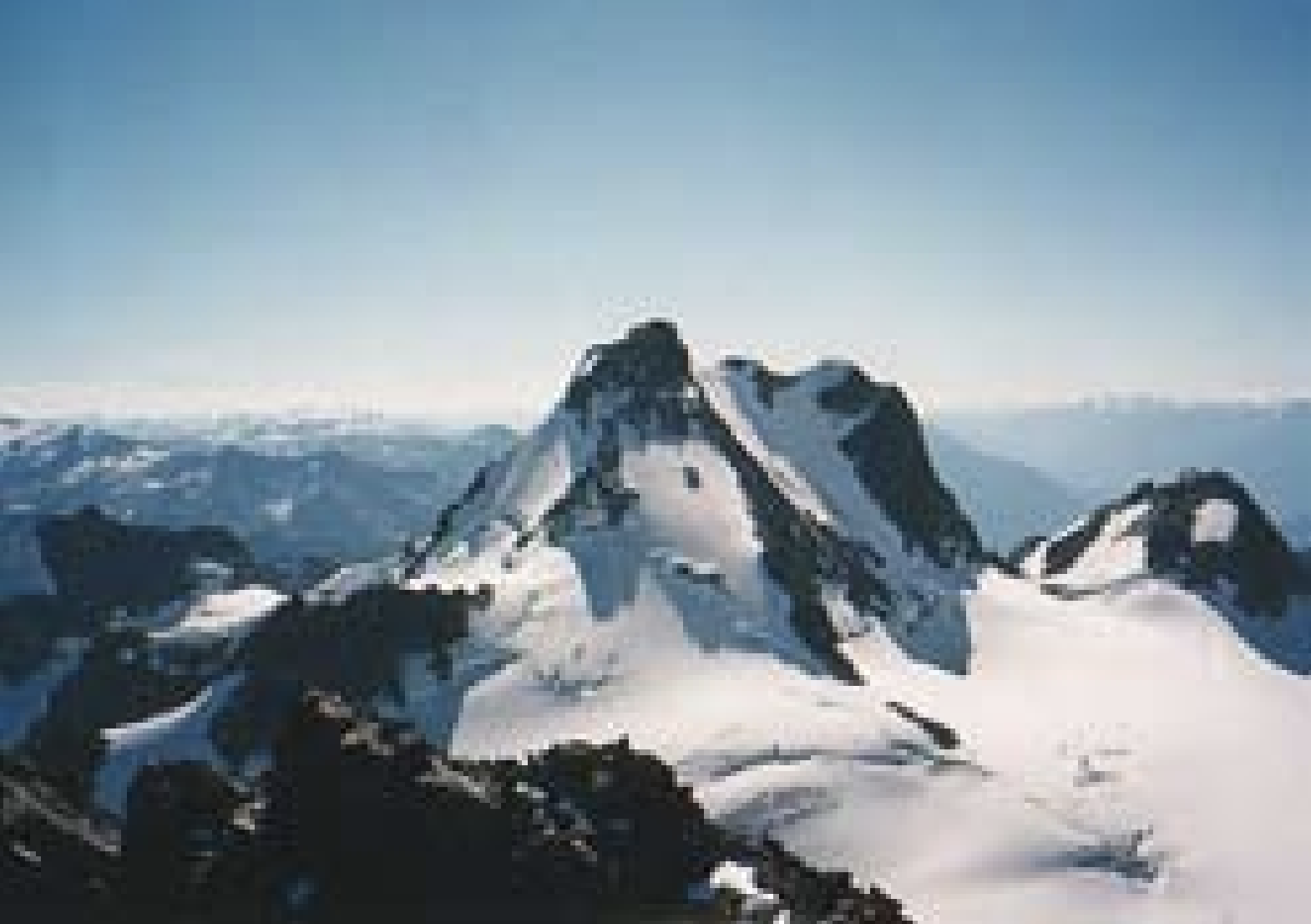
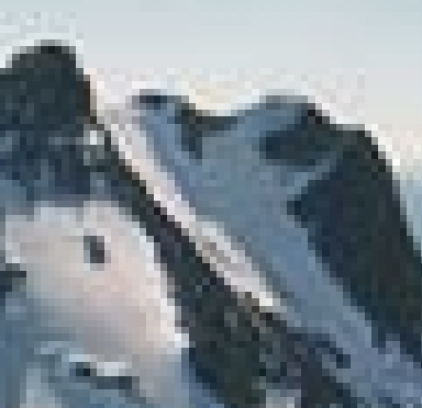
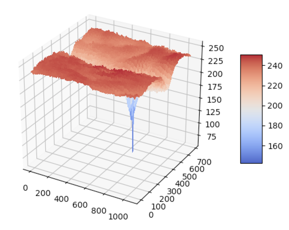
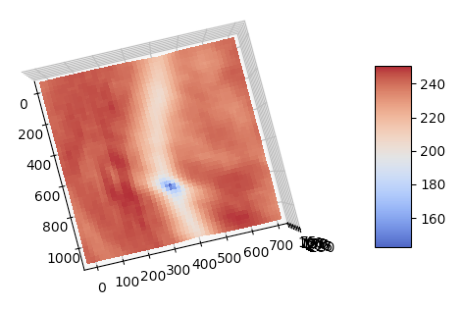
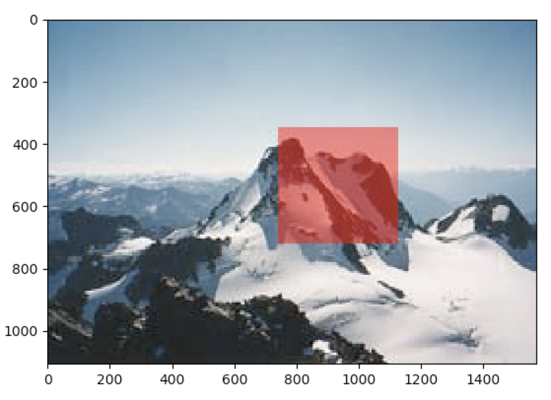
However, this method is unbelievable slow – it took 25 minutes even to localize this simple patch within an image.

When performing keypoint detection, we want to match local patches between images. However, we don’t know which local patches are the most informative, so we compute an “informativeness” score: how stable the WSSD function is with respect to small variations in position (\(\Delta \mathbf{u}\)).

Taylor Approximation: The Autocorrelation Matrix

Unfortunately, it turns out that the autocorrelation function is extraordinarily slow to evaluate.

The \(*\) in the equation you’ve written is not multiplication – it is convolution. Szeliski [1] states that he has “replaced the weighted summations with discrete convolutions with the weighting kernel \(w\)”.

So before we had values \(w(x,y)\) that could have been values from a Gaussian probability density function. Let \(z = \begin{bmatrix} x \\ y \end{bmatrix}\) be the stacked 2D coordinate locations.

For example, where \(\mu\) is the center pixel location and \(z\) is the location of each pixel in the local neighborhood. These were used as weights in summations over a local neighborhood,

But the elegant convolution approach is used here because it is equivalent to summing a bunch of elementwise multiplications – each point in a local neighborhood with its weight value (as we saw in Proj 1, and here filtering is equivalent to convolution since Gaussian filter is symmetric).

The Harris Corner Detector

A gaussian filter is expressed as \(g(\sigma_1)\).

The second moment matrix at each pixel is convolved as follows: \(\mu(\sigma_1,\sigma_D) = g(\sigma_1) * \begin{bmatrix} I_x^2 (\sigma_D) & I_xI_y (\sigma_D) \\ I_xI_y (\sigma_D) & I_{y}^2 (\sigma_D) \end{bmatrix}\) Giving a cornerness function in the lecture slides: \(har = \mbox{ det }[\mu(\sigma_1,\sigma_D)] - \alpha[\mbox{trace }\Big(\mu(\sigma_1,\sigma_D)\Big)]\)

or, when evaluated,

So in the lecture slides notation, we can write \(\mu(\sigma_1,\sigma_D)\) more simply by bringing in the filtering (identical to convolution here) operation:

It may be easier to understand if we write the equation in the following syntax:

I should have explained that above – \(\odot\) is the Hadamard product (element wise multiplication).

References

[1] Richard Szeliski. Computer Vision: Algorithms and Applications. PDF.

[2] Fei-Fei Li. PDF.

[3] Chris Harris and Mike Stephens. A Combined Edge and Corner Detector. PDF.