Generative Adversarial Networks (GANS)
Table of Contents:
- Overview
- Visual Interpretation: Generator and Discriminator
- Derivation of Losses
- Pytorch Implementation
- DCGAN Samples: CIFAR-10
- Advanced Topics
Overview
Generative Adversarial Networks (GANs) are a type of generative model that was popular between 2014 and 2022, but have since fallen out of fashion for a number of reasons. They are typically unstable and difficult to train, collapsing without carefully selected hyperparameters and regularizers (Dhariwal et al, 2021). Traditionally, GANS have also had low sample diversity compared to diffusion models, excelling only on a single category, such as human faces, although the recent GigaGAN (Kang, 2023), is an exception.
While GANs allow us to draw samples from a distribution \(p(x)\), computing likelihoods (density estimation) for samples \(x\) is not supported, except under some hacky approximations like kernel density estimation (KDE) / Parzen window estimation.
Visual Interpretation: Generator and Discriminator
GANs include a generator \(G\) and discriminator \(D\), both of which are trained with simple binary cross entropy losses. This loss is applied in three separate stages, and these three stages are repeated in each training iteration:

Derivation of Losses
Such a binary cross entropy (BCE) loss, which is available in Pytorch as the BCELoss, is defined as follows:
The three separate stages where this BCE loss is applied are defined as follows:
Stage 1A: Updating \(D\) with real data \(x\), and label \(y=1\):
\[\begin{aligned} \ell(x,y) &= -\Big[ 1 \cdot \log D(x) + (1-1) \cdot \log(1- D(x) )\Big] \\ &= -\Big[ 1 \cdot \log D(x) + 0 \Big] \\ &= -\log D(x) \end{aligned}\]Stage 1B: Updating \(D\) with fake data \(z\), and label \(y=0\):
\[\begin{aligned} \ell(z,y) &= -\Big[ 0 \cdot \log D(G(z)) + (1-0) \cdot \log(1- D(G(z)) )\Big] \\ &= -\Big[ 0 + (1) \cdot \log(1- D(G(z)) )\Big] \\ &= -\log (1-D(G(z))) \end{aligned}\]Algorithm 1 of the original GAN paper (Goodfellow et al., 2014) describes Stages 1a & 1b as gradient ascent, with a flipped sign: “Update the discriminator by ascending its stochastic gradient”:
\[\nabla_{\theta_d} \frac{1}{m} \sum_{i=1}^m \left[ \log D\left(\mathbf{x}^{(i)}\right) + \log \left(1-D\left(G\left(\mathbf{z}^{(i)}\right)\right)\right) \right].\]Stage 2: Updating \(G\) with fake data \(z\), and label \(y=1\) (ensure samples have high probability of being real)
\[\begin{aligned} \ell(z,y)_{non-saturating} &= -\Big[ 1 \cdot \log D(G(z)) + (1-1) \cdot \log(1- D(G(z)) )\Big] \\ &= -\Big[ 1 \cdot \log D(G(z)) + 0 \Big] \\ &= -\log D(G(z)) \end{aligned}\]This is the non-saturating version of the loss, as alluded to in the original GAN paper (Goodfellow et al., 2014) and in (Fedus et al., 2018), and implemented in DCGAN. In the minimax version of the loss, instead of minimizing the loss (penalizing when fake data is not assigned a label of 1), we could maximize the following loss through gradient ascent (ensure samples have low probability of being fake, i.e. being assigned a label \(y=0\)):
\[\begin{aligned} \ell(x,y)_{minimax} &= -\Big[ y \cdot \log x + (1-y) \cdot \log(1-x)\Big] \\ &= -\Big[ 0 \cdot \log D(G(z)) + (1-0) \cdot \log(1- D(G(z)) )\Big] \\ &= -\Big[ 0 + 1 \cdot \log(1- D(G(z)) )\Big] \\ &= -\log(1- D(G(z)) ) \end{aligned}\]Equivalently, instead of using gradient ascent, we could invert the sign and use gradient descent as follows:
\[\nabla_{\theta_g} \frac{1}{m} \sum_{i=1}^m \log \left(1-D\left(G\left(\mathbf{z}^{(i)}\right)\right)\right)\]Note this is not equal to what we described as Stage 2. The minimax version is indicated in Algorithm 1 of the original GAN paper (Goodfellow et al., 2014), described as “updat[ing] the generator by descending its stochastic gradient”.
As discussed in (Goodfellow et al., 2014), “in practice, the [minimax loss] may not provide sufficient gradient for \(G\) to learn well. Early in learning, when \(G\) is poor, \(D\) can reject samples with high confidence because they are clearly different from the training data. In this case, \(\log ( 1- D(G(\mathbf{z})))\) saturates. Rather than training \(G\) to minimize \(\log (1 - D(G(\mathbf{z})))\) we can train \(G\) to maximize \(\log D(G(\mathbf{z}))\). This objective function results in the same fixed point of the dynamics of \(G\) and \(D\) but provides much stronger gradients early in learning.”
Pytorch Implementation
We’ll now examine an implementation of a specific type of GAN, the DCGAN (Radford et al, 2015), in Pytorch, following the official example here.
- Sample minibatch of \(m\) examples \(\{ \mathbf{x}^{(1)}, \dots, \mathbf{x}^{(m)} \}\) from data generating distribution \(p_\text{data}(\mathbf{x})\)
- Sample minibatch of \(m\) noise samples \(\{ \mathbf{z}^{(1)}, \dots, \mathbf{z}^{(m)} \}\) from noise prior \(p_g(\mathbf{z})\)
criterion = nn.BCELoss()

fixed_noise = torch.randn(opt.batchSize, nz, 1, 1, device=device)
real_label = 1
fake_label = 0
Next, we’ll set up two optimizers. The gradient-based updates can use any standard gradient-based learning rule. Goodfellow et al. used momentum-based optimizers. We’ll use Adam:
optimizerD = optim.Adam(netD.parameters(), lr=opt.lr, betas=(opt.beta1, 0.999))
optimizerG = optim.Adam(netG.parameters(), lr=opt.lr, betas=(opt.beta1, 0.999))

for epoch in range(opt.niter):
    for i, data in enumerate(dataloader, 0):
        # ...Training loop logic...
We’ll now define the training loop logic. In Stage 1A:
############################
# Update D network: maximize log(D(x)) + log(1 - D(G(z)))
###########################
# train with real
netD.zero_grad()
real_cpu = data[0].to(device)
batch_size = real_cpu.size(0)
label = torch.full((batch_size,), real_label,
                   dtype=real_cpu.dtype, device=device)

output = netD(real_cpu)
errD_real = criterion(output, label)
errD_real.backward()
D_x = output.mean().item()
In Stage 1B:
# train with fake
noise = torch.randn(batch_size, nz, 1, 1, device=device)
fake = netG(noise)
label.fill_(fake_label)
output = netD(fake.detach())
errD_fake = criterion(output, label)
errD_fake.backward()
D_G_z1 = output.mean().item()
errD = errD_real + errD_fake
optimizerD.step()
In Stage 2:
############################
# Update G network: maximize log(D(G(z)))
###########################
netG.zero_grad()
label.fill_(real_label)  # fake labels are real for generator cost
output = netD(fake)
errG = criterion(output, label)
errG.backward()
D_G_z2 = output.mean().item()
optimizerG.step()
DCGAN Samples: CIFAR-10
CIFAR real image samples resemble the following:

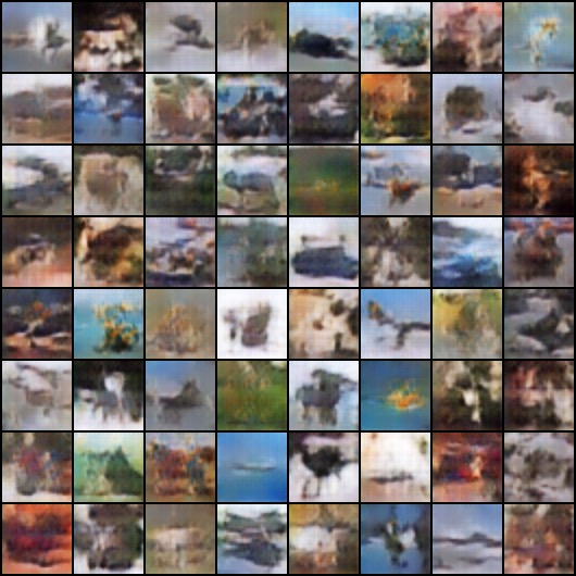
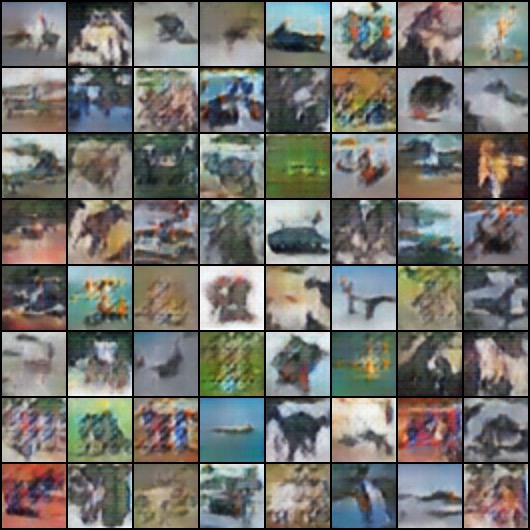
Below we visualize samples from each epoch of 25 epochs of training. You can see that mode collapse occurs at some epochs, such as Epoch 21 and Epoch 24, where weird artifacts arise. Epochs 22 and 23 have the best samples:

Epoch 0

Epoch 1

Epoch 2

Epoch 3

Epoch 4
Epoch 5
Epoch 6

Epoch 7

Epoch 8

Epoch 9

Epoch 10

Epoch 11

Epoch 12

Epoch 13

Epoch 14

Epoch 15

Epoch 16

Epoch 17

Epoch 18

Epoch 19

Epoch 20

Epoch 21

Epoch 22

Epoch 23

Epoch 24
We’ll print out:
print(
    f'[{epoch}/{opt.niter}][{i}/{len(dataloader)}] Loss_D: {errD.item():.4f}'
    f'Loss_G: {errG.item():.4f} D(x): {D_x:.4f} D(G(z)): {D_G_z1:.4f} / {D_G_z2:.4f}'
)
How does the minimax game start?
Discriminator losses start high, over 1.0.
[0/1][0/782] Loss_D: 1.7459 Loss_G: 7.1498 D(x): 0.6987 D(G(z)): 0.6811 / 0.0012
[0/1][1/782] Loss_D: 1.1919 Loss_G: 4.4647 D(x): 0.5069 D(G(z)): 0.2282 / 0.0147
[0/1][2/782] Loss_D: 1.5491 Loss_G: 5.6546 D(x): 0.7551 D(G(z)): 0.6141 / 0.0056
[0/1][3/782] Loss_D: 0.8161 Loss_G: 6.5825 D(x): 0.7683 D(G(z)): 0.3289 / 0.0020
[0/1][4/782] Loss_D: 0.9060 Loss_G: 6.2199 D(x): 0.6921 D(G(z)): 0.3113 / 0.0029
[0/1][5/782] Loss_D: 1.1162 Loss_G: 6.9918 D(x): 0.7187 D(G(z)): 0.3982 / 0.0015
[0/1][6/782] Loss_D: 0.8215 Loss_G: 7.2788 D(x): 0.7482 D(G(z)): 0.2837 / 0.0011
[0/1][7/782] Loss_D: 0.9057 Loss_G: 8.2282 D(x): 0.7596 D(G(z)): 0.3537 / 0.0005
[0/1][8/782] Loss_D: 1.0061 Loss_G: 7.2204 D(x): 0.6634 D(G(z)): 0.1923 / 0.0013
How does the minimax game end?
Discriminator losses end low, below 0.02.
[24/25][775/782] Loss_D: 0.0194 Loss_G: 10.8812 D(x): 0.9814 D(G(z)): 0.0001 / 0.0000
[24/25][776/782] Loss_D: 0.0261 Loss_G: 7.3836 D(x): 0.9762 D(G(z)): 0.0011 / 0.0010
[24/25][777/782] Loss_D: 0.0187 Loss_G: 8.1597 D(x): 0.9865 D(G(z)): 0.0003 / 0.0006
[24/25][778/782] Loss_D: 0.0039 Loss_G: 7.0521 D(x): 0.9975 D(G(z)): 0.0014 / 0.0019
[24/25][779/782] Loss_D: 0.0040 Loss_G: 8.1690 D(x): 0.9964 D(G(z)): 0.0004 / 0.0005
[24/25][780/782] Loss_D: 0.0111 Loss_G: 5.6885 D(x): 0.9991 D(G(z)): 0.0101 / 0.0057
[24/25][781/782] Loss_D: 0.0100 Loss_G: 8.0100 D(x): 0.9909 D(G(z)): 0.0005 / 0.0006
Advanced Topics
To obtain high-resolution samples with GANs, many additional tricks are needed. StyleGAN (Karras, 2018) and GigaGAN (Kang, 2023) describe these in detail.
References
[1]. Ian J. Goodfellow, Jean Pouget-Abadie, Mehdi Mirza, Bing Xu, David Warde-Farley, Sherjil Ozair, Aaron Courville, Yoshua Bengio. Generative Adversarial Networks. 2014. [PDF].
[2]. William Fedus, Mihaela Rosca, Balaji Lakshminarayanan, Andrew M. Dai, Shakir Mohamed, Ian Goodfellow. Many Paths to Equilibrium: GANs Do Not Need to Decrease a Divergence At Every Step. 2018. [PDF].
[3]. Alec Radford, Luke Metz, Soumith Chintala. Unsupervised Representation Learning with Deep Convolutional Generative Adversarial Networks. 2015. [PDF].
[4]. Tero Karras, Samuli Laine, Timo Aila. A Style-Based Generator Architecture for Generative Adversarial Networks. 2018. [PDF].
[5]. Minguk Kang, Jun-Yan Zhu, Richard Zhang, Jaesik Park, Eli Shechtman, Sylvain Paris, Taesung Park. Scaling up GANs for Text-to-Image Synthesis. 2023. [PDF].