Understanding Softmax Cross Entropy
Table of Contents:
Measures of Information
Common measures of information include entropy, mutual information, joint entropy, conditional entropy, and the s Kullback-Leibler (KL) divergence (also known as relative entropy).
Surprise
Let \(U\) be a discrete random variable, taking values in \({\mathcal U} = \{ u_1, u_2, \dots, u_M\}\). The Surprise Function \(S(u)\) is defined as
\[S(u) = \log_2 \Big( \frac{1}{p(U=u)} \Big) = \log_2 \Big( \frac{1}{p(u)} \Big)\]To make that more concrete,
surprise = lambda x: np.log2(1./x)
p_u = np.linspace(0,1,11)
We obtain probability values \(p(u)\), from small to large:
p_u
array([0. , 0.1, 0.2, 0.3, 0.4, 0.5, 0.6, 0.7, 0.8, 0.9, 1. ])
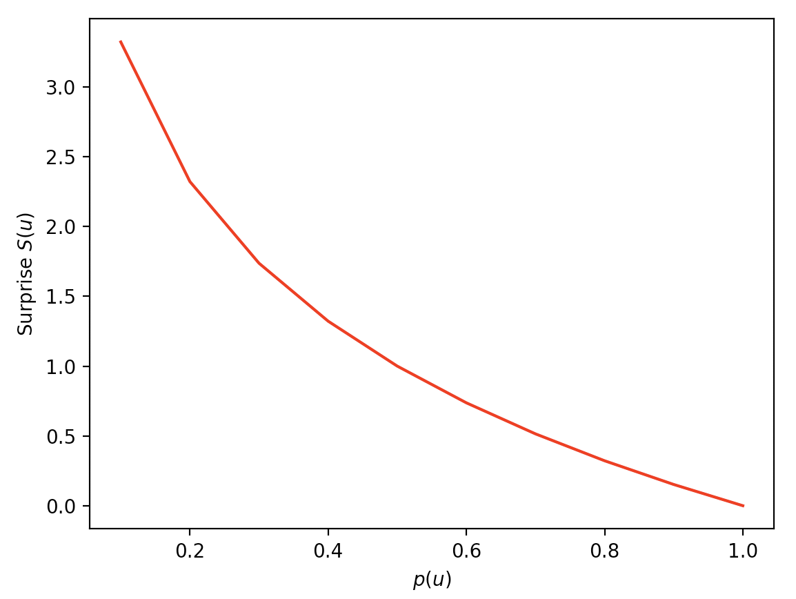
and surprise values that decrease as \(p(u)\) increases:
array([ inf, 3.32, 2.32, 1.74, 1.32, 1. , 0.74, 0.51, 0.32, 0.15, 0. ])
We can plot the values:
import matplotlib.pyplot as plt
plt.plot(p_u,S,'r')
plt.xlabel(r'$p(u)$')
plt.ylabel(r'Surprise $S(u)$')
plt.show()

Entropy
The entropy of \(U\) is simply the expected Surprise. More formally,
\[\begin{aligned} H(U) &= \mathbb{E}[S(U)] \\ &= \mathbb{E}\Big[\log_2\big(\frac{1}{p(U)}\big)\Big] \\ &= \mathbb{E}\Big[\log_2\big(p(U)^{-1}\big)\Big] \\ &= \mathbb{E}\Big[-\log_2 p(U)\Big] & \text{because } \log x^{k} = k \log x \\ &= - \sum\limits_u p(u) \log_2 p(u) & \text{by definition of expectation} \end{aligned}\]Thus, entropy measures the amount of surprise or randomness in the random variable [1].
Consider the entropy of 3 simple distributions over \({\mathcal U} = \{ u_1, u_2, u_3, u_4\}\), and their probability masses \([p(U=u_1),p(U=u_2),p(U=u_3),p(U=u_4)]\).
cross_entropy = lambda x: -np.sum(np.log2(x)*x)

p1 = np.array([0.97, 0.01, 0.01, 0.01])
surprise(p1)
array([0.04, 6.64, 6.64, 6.64])
The entropy of p1 is 0.24, since although we get some high surprise values, they have very little probability mass.
p2 = np.array([0.5,0.3, 0.19, 0.01])
surprise(p2)
array([1.  , 1.74, 2.4 , 6.64])
The entropy of p2 is 1.54, and once again, although we get one high surprise value, it has almost no probability mass: \(p(U=u_4)=0.01\).
p3 = np.array([0.25, 0.25, 0.25, 0.25])
surprise(p3)
array([2., 2., 2., 2.])
Finally, the entropy of p3 is 2.0. We get the most average surprise from p3 (a uniform distribution).
KL Divergence (Relative Entropy)
The Kullback-Leibler (KL) divergence, also known as relative entropy, is defined as
Cross Entropy
\[H(p,q) = - \sum_x p(x) \log q(x)\] \[H(p,q) = H(p) + D_{KL}(p||q)\]In PyTorch, the negative log likelihood loss (NLL loss) can be used for multinomial classification, and expects to receive log-probabilities for each class.
Consider an empirical output distribution [0.2, 0.6, 0.2] and a target distribution [0,1,0], in a one-hot format. The index of the target class is simply 1, which is the format PyTorch expects for the target. NLLLoss() expects log-probabilities:
nll = torch.nn.NLLLoss()
x = torch.tensor([[0.2, 0.6, 0.2]])
x = np.log(x)
y = torch.tensor([1])
loss = nll(x,y)
print(loss)
	tensor(0.5108, dtype=torch.float64)
Our goal is to minimize this quantity. We can do so by making the target and empirical distribution match more closely. When the two distributions come closer and closer, the loss (divergence between them) decreases:
for dist in [ [0.3, 0.4, 0.3], [0.2, 0.6, 0.2], [0.1, 0.8, 0.1], [0,1.,0] ]:
	nll = torch.nn.NLLLoss()
	x = torch.tensor([np.log(dist)])
	y = torch.tensor([1])
	loss = nll(x,y)
	print(loss)
In this case, 0.9163, 0.5108, 0.2231, 0. is printed, meaning the loss drops as the distributions align, until it finally reaches zero when the distributions are identical.
(torch.nn.CrossEntropyLoss incorporates torch.nn.LogSoftmax inside of it).
Logistic Regression
Consider a binary (two-class) classification problem. Here \(y\) can take on the values \(\{0,1\}\). A common real-world example is a spam classifier for email, where \(x\) denotes features for an email, and \(y\) is 1 if it is a piece of spam mail [2], and 0 otherwise. We call \(y\) the label for the training example.
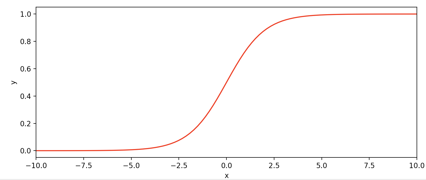
Since we wish to train a model to output probabilities \(p\) in the range \([0,1]\), where \(p>0.5\) might indicate a prediction that \(y=1\), we will use a function with that exact range (the sigmoid or logistic function):
\[g(z) = \sigma(z) = \frac{1}{1 + e^{-z}}\]import numpy as np
import matplotlib.pyplot as plt
g = lambda z: 1. / ( 1+ np.exp(-z))
x = np.linspace(-10,10,100)
y = g(x)
plt.plot(x,y,'r-')
plt.xlim([-10,10])
plt.xlabel('x')
plt.ylabel('y')
plt.show()

Note that \(g(z)\) tends towards 1 as \(z \rightarrow \infty\), and \(g(x)\) tends toward 0 as \(z \rightarrow -\infty\). Our hypothesis class will be
\[h_{\theta}(x) = g(\theta^Tx) = \sigma(\theta^Tx) = \frac{1}{1 + e^{-\theta^Tx}}\]Since \(g(z)\) is bounded between \([0,1]\), then \(h(x)\) will also be bounded. In order to fit a model, we need to learn a set of weights \(\theta\) from data. We can do so by identifying a set of probabilistic assumptions and ffiting the model via maximum likelihood estimation (MLE) [2]. Let us assume that two events are possible: either \(y=1\), or \(y=0\). The probability of the second event is equal to the complement of the probability of the first event, thus:
\[\begin{aligned} P(y = 1 \mid x; \theta) = h_{\theta}(x) \\ P(y = 0 \mid x; \theta) = 1 - h_{\theta}(x) \end{aligned}\]A beautiful way to combine these two expressions is as follows:
\[p(y \mid x; \theta) = \Big( h_{\theta}(x)\Big)^y \Big(1 - h_{\theta}(x)\Big)^{1-y}\]We note that as desired, if \(y=0\), then \(p(y=0 \mid x; \theta) = h_{\theta}(x)^0 \Big(1 - h_{\theta}(x)\Big)^{1-0} = 1 \cdot (1 - h_{\theta}(x))\).
Also, if \(y=1\), then \(\Big( h_{\theta}(x)\Big)^1 \Big(1 - h_{\theta}(x)\Big)^{0} = h_{\theta}(x) \cdot 1\), as desired.
If we assume that \(m\) training example were generated independently, then their joint probability is equal to the product of the probability of each independent event [2]. Let \(\vec{y}\) denote a column vector with stacked \(y^{(i)}\) entries, and let \(X\) denote a matrix with stacked \(x^{(i)}\) entries. Then the likelihood is:
\[\begin{aligned} L(\theta) &= p(\vec{y} \mid X; \theta) \\ &= \prod_{i=1}^m p( y^{(i)} \mid x^{(i)}; \theta ) \\ &= \prod_{i=1}^m \big( h_{\theta}(x^{(i)}) \big)^{y^{(i)}} \Big( 1 - h_{\theta}(x^{(i)}) \Big)^{1 - y^{(i)}} \end{aligned}\]Maximizing the log-likelihood is easier, and we recall that the log of a product is a sum of logs:
\[\begin{aligned} \ell(\theta) &= \log L(\theta) \\ &= \log \Bigg( \prod_{i=1}^m \big( h_{\theta}(x^{(i)}) \big)^{y^{(i)}} \Big( 1 - h_{\theta}(x^{(i)}) \Big)^{1 - y^{(i)}} \Bigg) \\ &= \sum_{i=1}^m \log \Bigg( \big( h_{\theta}(x^{(i)}) \big)^{y^{(i)}} \Big( 1 - h_{\theta}(x^{(i)}) \Big)^{1 - y^{(i)}} \Bigg) & \mbox{log of a product is a sum of logs} \\ &= \sum_{i=1}^m \log \big( h_{\theta}(x^{(i)}) \big)^{y^{(i)}} + \log \Big( 1 - h_{\theta}(x^{(i)}) \Big)^{1 - y^{(i)}} & \mbox{log of a product is a sum of logs} \\ &= \sum\limits_{i=1}^m y^{(i)} \log h_{\theta}(x^{(i)}) + (1-y^{(i)}) \log \big(1-h_{\theta}(x^{(i)})\big) & \mbox{because } \log(M^k) = k \cdot \log M \end{aligned}\]We can maximize the likelihood in this case by gradient ascent, equivalent to minimizing the negative log likelihood, \(-\ell(\theta)\).
\[NLL(\theta) = -\ell(\theta) = \sum\limits_{i=1}^m y^{(i)} \log h_{\theta}(x^{(i)}) + (1-y^{(i)}) \log \big(1-h_{\theta}(x^{(i)})\big)\]The Sigmoid / Binary Cross Entropy (BCE) Loss
As described in the TensorFlow docs, the logistic regression loss (often called sigmoid loss or binary cross entropy loss) can be used to measure the probability error in discrete classification tasks in which each class is independent and not mutually exclusive. For instance, one could perform multilabel classification where a picture can contain both an elephant and a dog at the same time. In PyTorch, there are two options for this loss: one with the sigmoid output, and one with the sigmoid input.
torch.nn.BCELoss accepts the sigmoid output \(h^{(i)}\), not \(x^{(i)}\), where \(h^{(i)} = h_{\theta}(x^{(i)}) = \sigma(\theta^T x^{(i)})\):
torch.nn.BCEWithLogitsLoss accepts as input \(\theta^Tx^{(i)}\), and applies the sigmoid function to it.
Thus, torch.nn.BCEWithLogitsLoss combines a Sigmoid layer and the BCELoss in one single class.
Numerical Stability of the Sigmoid/BCE Loss
https://www.tensorflow.org/api_docs/python/tf/nn/sigmoid_cross_entropy_with_logits
Softmax Regression
(Section 9.3 Softmax Regression of [2]).
The Softmax Operation
soft = nn.Softmax(dim=1)
x = torch.tensor([[0,1,2],[0.8, 0.4, 0.4]])
x = soft(x)
print(x)
The first row can identically be computed by:
x = np.array([0,1,2])
x = np.exp(x)
x = x / np.sum(x)
print(x)
Consider the Negative Log Likelihood (NLL) loss criterion.
References
[1] Tsachy Weissman. Information Theory (EE 376, Stanford) Course Lectures. PDF.
[2] Andrew Ng. CS229 Lecture notes. PDF.