Convex Optimization Without the Agonizing Pain
Convexity
First-Order Condition
If \(f\) is convex and differentiable, then
\[f(x) + \nabla f(x)^T (y-x) \leq f(y)\]That is to say, a tangent line to \(f\) is a global underestimator of the function.
Second-Order Condition
Assuming \(f\) is twice differentiable, that is, its Hessian or second derivative \(\nabla^2f\) exists at each point in the domain of \(f\), then \(f\) is convex **if and only if ** the domain of \(f\) is convex and its Hessian is positive semidefinite.
Formally, we state, for all \(x \in \mbox{dom}(f)\),
\(\nabla^2 f(x) \succeq 0\) This condition can be interpreted geometrically as the requirement that the graph of the function have positive (upward) curvature at \(x\).
Known Convex and Concave Functions
Convex:
- Linear. A simple example is \(f^Tx\).
- Affine. \(f(x) = Ax+b\), where \(A \in \mathbb{R}^{m \times n}\) and \(b \in \mathbb{R}^m\). This is the sum of a linear function and a constant.
- Exponential. \(e^{ax}\) is convex on \(\mathbb{R}\), for any \(a \in \mathbb{R}\).
- Even powers \(x^2,x^4,x^6, \dots\) on \(\mathbb{R}\).
- Powers. \(x^a\) is convex on \(R_{++}\) when \(a \geq 1\) or \(a \leq 0\).
- Powers of absolute value. \(|x|^p\), for \(p\geq 1\), is convex on \(\mathbb{R}\).
- Negative Entropy. \(x \mbox{log}(x)\) is convex on \(\mathbb{R}_{++}\).
- Norms. Every norm \(\| \cdot \|\) on \(\mathbb{R}^n\) is convex.
- Max function. \(f(x) = \mbox{max } { x_1, \dots, x_n } \) is convex on \(\mathbb{R}^n\).
- Quadratic-over-linear function.
- Log-sum-exp. \(f(x) = \mbox{log }(e^{x_1}+\cdots+e^{x_n})\) is convex on \(\mathbb{R}^n\).
Concave:
- Logarithm. \(\mbox{log}(x)\) concave on \(\mathbb{R}_{++}\).
- Powers. \(x^a\) is concave for \(0 \leq a \leq 1\).
-
Geometric mean. \(f(x) = (\prod\limits_{i=1}^n x_i)^{1/n}\) is concave on \(\mathbb{R}_{++}^n\).
- Log-determinant. \(f(X) = \mbox{log } \mbox{det } X\) is concave on \(S_{++}^n\)
Calculus of Convex Functions [3]
Convexity-preserving operations:
- Taking conic combinations. If each \(f_i(x)\) is a convex function on \(\mathbb{R}^n\) and \(\lambda_i \geq 0\), then the function \(\sum\limits_i \lambda_i f_i(x)\) is convex.
- Affine substitution of an argument. If \(f(x)\) is a convex function on \(\mathbb{R}^n\) and \(x=Ay+b\) is an affine mapping from \(\mathbb{R}^k \rightarrow \mathbb{R}^n\), then the function \(g(y) = f(Ay+b)\) is convex on \(\mathbb{R}^k\).
- Taking the supremum of a family of convex functions (it is the intersection of two epigraphs, and epigraphs are convex sets)
Constrained Optimization Problems
These problems take on a very general form, that we’ll revisit over and over again. In math, that form is:
\[\begin{aligned} \begin{array}{lll} \mbox{minimize} & f_0(x) & \\ \mbox{subject to} & f_i(x) \leq 0, & i=1,\dots,m \\ & h_i(x) = 0, & i=1,\dots,p \end{array} \end{aligned}\]In prose, the problem is to find an \(x\) that minimizes \(f_0(x)\) among all \(x\) that satisfy the conditions \( f_i(x) \leq 0\) for \(i=1,\dots,m \) and \( h_i(x) = 0\) for \( i=1,\dots,p\).
The inequalities \(f_i(x) \leq 0\) are called inequality constraints, and the equations \(h_i(x) = 0\) are called the equality constraints.
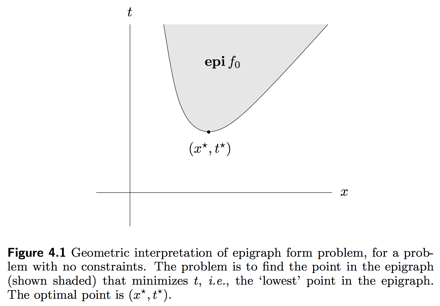
The Epigraph form of the above standard problem is the problem
\[\begin{aligned} \begin{array}{lll} \mbox{minimize} & t & \\ \mbox{subject to} & f_0(x) - t \leq 0 & \\ & f_i(x) \leq 0, & i=1,\dots,m \\ & h_i(x) = 0, & i=1,\dots,p \end{array} \end{aligned}\]Geometrically, from [1]:

The Lagrangian
The basic idea in Lagrangian duality is to take the constraints in the standard problem into account by augmenting the objective function with a weighted sum of the constraint functions. The Lagrangian associated with the standard problem is:
\[L(x, \lambda, \nu) = f_0(x) + \sum\limits_{i=1}^{m} \lambda_i f_i(x) + \sum\limits_{i=1}^p \nu_i h_i(x)\]We call \(\lambda_i\) as the Lagrange multiplier associated with the \(i\)’th inequality constraint \(f_i(x) \leq 0\). We refer to \(\nu_i\) as the Lagrange multiplier associated with the \(i\)’th equality constraint \(h_i(x) = 0\).
The Lagrange Dual Function
\[g(\lambda, \nu) = \underset{x \in \mathcal{D}}{\mbox{inf }} L(x,\lambda,\nu)\]In detail, the dual function is:
\[g(\lambda, \nu) = \underset{x \in \mathcal{D}}{\mbox{inf }}\Bigg( f_0(x) + \sum\limits_{i=1}^{m} \lambda_i f_i(x) + \sum\limits_{i=1}^p \nu_i h_i(x) \Bigg)\]This is the pointwise infimum of a family of affine functions of \( (\lambda, \nu)\), so the dual function is concave, even when the standard optimization problem is not convex.
The Lagrange Dual Problem
For each pair \( (\lambda, \nu)\), the Lagrange dual function gives us a lower bound on the optimal value \(p^{*}\) of the standard optimization problem. It is a lower bound that depends on some parameters \( (\lambda,\nu)\). But the question of interest for us is, what is the best lower bound that can be obtained from the Lagrange dual function. This leads to the following optimization problem:
\[\begin{aligned} \begin{array}{ll} \mbox{maximize} & g(\lambda, \nu) \\ \mbox{subject to} & \lambda \succeq 0 \end{array} \end{aligned}\]We refer to this problem as the Lagrange dual problem associated with the standard optimization problem.
Weak Duality
Let us define \( d^* \) as the optimal value of the Lagrange dual problem. This is the best lower bound on \( p^* \) that can be obtained from the Lagrange dual function.
Even if the original problem is not convex, we can always say \(d^* \leq p^*\). We call this property weak duality.
Slater’s Constraint Qualification
Slater’s condition is a qualification on the problem constraints. It states that there exists an \(x \in \mbox{relint}(\mathcal{D})\) such that
\[\begin{array}{lll} f_i(x) < 0, & i=1,\dots,m, & Ax=b. \end{array}\]Why is that important? Well, because if the problem is convex, and if Slater’s condition holds, then strong duality holds.
KKT Conditions (See[1] p. 243)
Let \(x^{\star}\) and \(\lambda^{\star}, \nu^{\star})\) be any primal and dual optimal points with “zero duality gap” (we will explain what this means shortly).
Since this is a feasible (and optimal) point, each of the \(p\) equality constraints must be fulfilled, meaning:
\[\begin{array}{ll} h_i(x^{\star}) = 0, i = 1, \dots, p \end{array}\]Also, we can certainly say that each of the inequality constraints \(f_i\) must also be fulfilled:
\[f_i(x^{\star}) \leq 0, i = 1, \dots , m\]The point \(x^{\star}\) minimizes \(L(x, \lambda^{\star}, \nu^{\star}\) over \(x\in \mathbb{R}^n\), so its gradient must vanish at \(x^{\star}\):
\[\nabla f_0(x^{\star}) + \sum\limits_{i=1}^m \lambda_i^{\star} \nabla f_i(x^{\star} ) + \sum\limits_{i=1}^p \nu_i^{\star} \nabla h_i(x^{\star}) = 0.\]Complementary Slackness
The next condition is called “complementary slackness”, which at first makes absolutely zero sense. However, I will explain it, from [1] and [2]
Suppose that primal and dual optimal values are attained and equal (so, in particular, strong duality holds). Let \(x^{\star}\) be a primal optimal and \( (\lambda^{\star}, \nu^{\star})\) be a dual optimal point. This means that
\[\begin{aligned} \begin{array}{ll} \mbox{primal value} = \mbox{dual value}, & (\mbox{ bc optimal duality gap is zero})\\ f_0(x^{\star}) = g(\lambda^{\star}, \nu^{\star}) & (\mbox{ by definitions of primal and dual function values})\\ = \underset{x}{\mbox{inf }} \Bigg(f_0(x) + \sum\limits_{i=1}^m \lambda_i^{\star} f_i(x) + \sum\limits_{i=1}^p \nu_i^{\star} h_i(x) \Bigg) & (\mbox{ by definition of the dual function})\\ \leq f_0(x^{\star}) + \sum\limits_{i=1}^m \lambda_i^{\star} f_i(x^{\star}) + \sum\limits_{i=1}^p \nu_i^{\star} h_i(x^{\star}) & \mbox{ (bc the infimum of the Lagrangian over } x \mbox{ is less than or equal to its value at } x = x^{\star} )\\ \leq f_0(x^{\star}) & (\mbox{ bc } \lambda_i^{\star} \geq 0, f_i(x^{\star}) \leq 0, i= 1,\dots,m \mbox{ and } h_i(x^{\star}) = 0, i = 1, \dots, p) \end{array} \end{aligned}\]This is a somewhat suprising result: all these inequalities are actually equalities.
We can safely conclude from this proof that the following term is zero:
\[\sum\limits_{i=1}^m \lambda_i^{\star} + f_i(x^{\star}) = 0.\]At the same time, we know that at \(x^{\star}\) our inequality constraints \(f_i(x^{\star}) \leq 0\) are all fulfilled (\(\forall i)\). Thus, combining this fact with the above result, we know that every single term in the sum must also equal zero:
\[\lambda_i^{\star} f_i(x^{\star}) = 0, i = 1, \dots , m\]This is complementary slackness.
Finally, the Lagrange dual required that each element of \(\mathbf{\lambda}\) be positive:
\[λ_i^{\star} \geq 0, i = 1, \dots , m\]We call these 5 conditions the Karush-Kuhn-Tucker (KKT) conditions. In short, If \(x^{\star}\) and \(u^{\star}, v^{\star}\) are primal and dual solutions, with zero duality gap, then \(x^{\star}, \lambda^{\star}, \nu^{\star}\) satisfy the KKT conditions.
In stating this, we have assumed nothing a priori about convexity of our problem, i.e. of \(f_0, f_i, h_i\).
Simple Example with Matrix-vector product (See [2])
Consider for \(Q \succeq 0\) (i.e. positive semidefinite),
\[\begin{array}{ll} \underset{x \in \mathbb{R}^n}{\mbox{min}} & \frac{1}{2}x^TQx + c^Tx \\ \mbox{subject to} & Ax = 0 \end{array}\]This is a convex problem, so by the KKT conditions, \(x\) is a solution iff
\[\nabla L(x,\lambda) = \nabla \Bigg(\frac{1}{2}x^TQx + c^Tx + \lambda^T (Ax) \Bigg) = 0 \\\]For \(\nabla_x\), \( Qx + c + A^T \lambda = 0 \).
For \(\nabla_{\lambda}\), \(Ax=0\).
This system of equations can be written in matrix form as:
\[\begin{bmatrix} Q & A^T \\ A & 0 \end{bmatrix} \begin{bmatrix} x \\ \lambda \end{bmatrix} = \begin{bmatrix} -c \\ 0 \end{bmatrix}\]for some \(\lambda\).
Newton’s Method
Instead of minimizing the first-order Taylor approximation of a function \(f\), we may want to minimize the second-order Taylor approximation, \(f^k(\mathbf{x})\). That approximation around a point \(\mathbf{x}^k\) is given by:
\[f^k(\mathbf{x}) = f(\mathbf{x}^k) + \nabla f(\mathbf{x}^k)^T (\mathbf{x}-\mathbf{x}^k) + \frac{1}{2}(\mathbf{x}-\mathbf{x}^k)^T \nabla^2 f(\mathbf{x}^k) (\mathbf{x}-\mathbf{x}^k)\]By setting derivative w.r.t \(\mathbf{x}\) to 0, we find:
\[\nabla f(\mathbf{x}^k) + \nabla^2 f(\mathbf{x}^k) (\mathbf{x} - \mathbf{x}^k) = 0\]Multiply all terms on the left by the inverse of the Hessian, \(H^{-1}= (\nabla^2 f)^{-1} \),
\[(\nabla^2 f)^{-1} \nabla f(\mathbf{x}^k) + (\mathbf{x}-\mathbf{x}^k) = 0\]\(\mathbf{x} = \mathbf{x}^{k} - (\nabla^2 f)^{-1} \nabla f(\mathbf{x}^k)\) The expression you may be familiar with for a Newton step is:
\[\mathbf{x}^{k+1} = \mathbf{x}^{k} - \frac{ \nabla f(\mathbf{x}^k) }{(\nabla^2 f)}\]However, a Newtons step requires not only the computation of the Hessian, but also being able to invert it. Thus, one may need to regularize \(H=\nabla^2 f\) so that your Hessian \(H\) is invertible (if the Hessian is not positive definite).
If the function \(f\) is quadratic, then minimizing the 2nd order Taylor approximation given above, \(f^k\), will give us an exact minimizer of \(f\). If the function \(f\) is nearly quadratic, intuition suggests that minimizing this 2nd order expansion should be a very good estimate of the minimizer of \(f\), i.e., \(x^*\).
Interior Point Methods
Suppose we have the following inequality constrained optimization problem:
We can approximate the problem as an equality constrained problem. This is highly desirable because we know that Newton’s method can be applied to equality constrained problems. We can make the inequality constraints implicit in the objective:
\[\begin{aligned} \begin{array}{lll} \mbox{minimize} & f_0(x) + \sum\limits_{i=1}^m I_{-}\bigg(f_i(x)\bigg) & \\ \mbox{subject to} & Ax = b \end{array} \end{aligned}\]The indicator function expresses our displeasure with respect to the satisfaction of the inequality constraints. If the indicator function is violated, its value becomes negative infinity:
\[I_{-}(u) = \begin{cases} 0 & u\leq 0 \\ \infty & u > 0 \end{cases}\]Otherwise, we ignore its presence in the objective function. Although we were able to remove the inequality constraints, the objective function is, in general, not differentiable, so Newton’s method cannot be applied.
The Log-Barrier
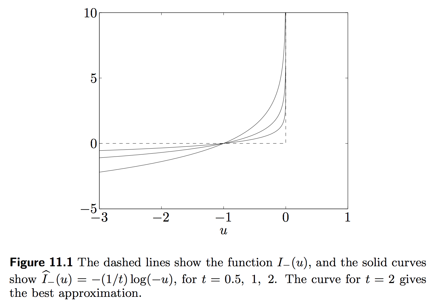
However, we could approximate the indicator function \(I_{-}\) with the log-barrier function:
\[\hat{I}_{-}(u) = -\bigg(\frac{1}{t}\bigg) \mbox{log }(-u)\]Here, \(t\) is a parameter that sets the accuracy of the approximation. As \(t\) increases, the approximation becomes more accurate.
A figure shows the quality of the approximation [1]:

We now have a new problem:
\[\begin{aligned} \begin{array}{lll} \mbox{minimize} & f_0(x) + \sum\limits_{i=1}^m -\bigg(\frac{1}{t}\bigg) \mbox{log }\bigg(-f_i(x)\bigg) & \\ \mbox{subject to} & Ax = b \end{array} \end{aligned}\]This objective function is convex, and as long as an appropriate closedness condition holds, Newton’s method can be used to solve it.
References:
-
Stephen Boyd and Lieven Vandenberghe. 2004. Convex Optimization. Cambridge University Press, New York, NY, USA.
-
Gordon, Geoff. CMU 10-725 Optimization Fall 2012 Lecture Slides, Lecture 16.
-
Arkadiy Nemirovski