Modern Iterative Methods for Linear System Solving
Table of Contents:
Modern Iterative Solvers for Systems of Linear Equations
Two key ideas serve as the foundation of modern iterative solvers: Krylov subspaces and pre-conditioning. In this tutorial, we’ll discuss Krylov subspaces for the problem \(Ax=b\).
The Krylov Subspace
CG relies upon an idea named the Krylov subspace. The Krylov subspace is defined as the span of the vectors generated from successively higher powers of \(A\):
\[\mathcal{K}_k = \mbox{span} \{b, Ab, \dots, A^{k-1}b \}\]Krylov subspace approximation is a hierarchical (nested) structure of subspaces. We will search for an approximation of \(x\) in this space. A first approximation is \(x_0 \in \mbox{span} \{ \vec{b} \}\). If \(A\) is the identity matrix or a scalar, then this subspace is already sufficient to find \(x\) in \(Ax=b\).
We can proceed with higher powers of \(k\), e.g. \(x_1 \in \mbox{span} \{b, Ab \}\), \(x_k \in \mbox{span} \{ b, Ab, \cdots, A^{k-1}b \}\). Our approximation for \(x^{\star}\) will become increasingly refined as we perform enlargement of Krylov subspaces.
The Krylov sequence is a sequence of solutions to our convex objective \(f(x)\). Each successive solution has to come from a subspace \(\mathcal{K}_k\) of progressively higher power \(k\). Formally, the Krylov sequence \(x^{(1)},x^{(2)},\dots\) is defined as:
\[x^{(k)} = \underset{x \in \mathcal{K}_k}{\mbox{argmin }} f(x)\]The CG algorithm generates the Krylov sequence. The beauty of the Krylov subspaces are that any element (a vector) can be constructed only with (1) matrix vector multiplication, (2) vector addition, and (3) vector-scalar multiplication. We never have to compute expensive things like \(A^{-1}\), or determinant. This is because \(Ab\) is a vector, so \(A^2b = A(Ab)\) is also just matrix-vector multiplication of \(A\) with the vector \(Ab\).
Theorem: Justification of Krylov Subspaces
Theorem: Given any nonsingular \(A\) of shape \({n \times n}\), then
\[A^{-1}b \in \mbox{span} \Bigg\{ b, Ab, A^b, \cdots, A^{n-1}b \Bigg\} = \mathcal{K}_n\]This theorem has two implications: (1) If you search inside \(\mathcal{K}_n\), whether or not \(K\) spans the whole space \(\mathbf{R}^{n}\), you will get the solution. An extreme case when \(K \neq \mathbf{R}^n\) is that \(b\) is an eigenvector of \(A\) (then the space is 1-dimensional). If you want to solve a linear system, this is why it is sufficient to look inside the Krylov subspaces. Implication 2: If you search orthogonally inside \(K\), then you can get the solution in \(\leq n\) steps. The Krylov subspace is at most $n$-dimensional since it is composed of \(n\)-dimensional vectors. CG, Orthomin(2), and GMRES all do this. GMRES is in a more general setup. Notice that the theorem itself is independent of the search algorithm – it will always be true. To prove the theorem, we need a lemma:
Lemma: The Cayley-Hamilton Theorem
Let \(\chi(s)\) be a polynomial function of \(s\) defined as \(\chi(s) = \mbox{det}(sI-A)\) which is the characteristic polynomial of \(A\). Then \(\chi(A)=0_{n \times n}\) (a zero matrix). The Cayley-Hamilton Theorem states that if \(A \in \mathbf{R}^{n \times n}\):
\[A^n + \alpha_1 A^{n-1} + \cdots + \alpha_n I = 0_{n \times n}\]We can solve for \(I\) by rearranging terms:
\[\alpha_n I = - A^n + - \alpha_1 A^{n-1} + \cdots + \alpha_{n-1} A^{1}\]We now divide by \(\alpha_n\):
\[I = - \frac{1}{\alpha_n} A^n + - \frac{\alpha_1}{\alpha_n} A^{n-1} + \cdots + \frac{\alpha_{n-1}}{\alpha_n} A^{1}\]We now left-multiply all terms by \(A^{-1}\) and simplify:
\[\begin{aligned} A^{-1}I & = - \frac{1}{\alpha_n} A^{-1} A^n + - \frac{\alpha_1}{\alpha_n} A^{-1} A^{n-1} + \cdots + \frac{\alpha_{n-1}}{\alpha_n} A^{-1} A^{1} \\ A^{-1} & = - \frac{1}{\alpha_n} A^{n-1} + - \frac{\alpha_1}{\alpha_n} A^{n-2} + \cdots + \frac{\alpha_{n-1}}{\alpha_n} I \\ \end{aligned}\]We can now see that \(x^{\star}\) is a linear combination of the vectors that span the Krylov subspace. Thus, \(x^{\star} = A^{-1}b \in \mathcal{K}_n\).
Thus, we need to search in the Krylov subspace of maximum size! If you have a smaller subapce, you may or may not have the exact solution inside.
Krylov Subspace Methods
We will consider two types of error. One:
\(r_k = b-Ax_k\) residue/residual: what your \(x_k\) cannot satisfy smaller \(\|r_k\| \implies\) better satisfaction of the equation $\approx$ better accuracy
Two, your error: \(e_k = x^{\star} - x_k\). These are not the same thing.
| Orthomin(1) | Orthomin(2) | |
|---|---|---|
| \(r_{k+1} = r_k - a_k A p_k\) | \(r_{k+1} \perp A p_k\) | \(r_{k+1}\) |
| \(e_{k+1} = e_k - a_k p_k\) | \(e_{k+1} \perp_A p_k\) | \(e_{k+1}\) |
Suppose we define some kind of iterative method via a recurrence relation:
\[\begin{aligned} x_{k+1} &= x_k + a_k (b- Ax_k) \\ x_{k+1} &= x_k + a_kr_k \end{aligned}\]We can then also obtain a recurrence between the residuals, with \(a_k\) as our scalar knob:
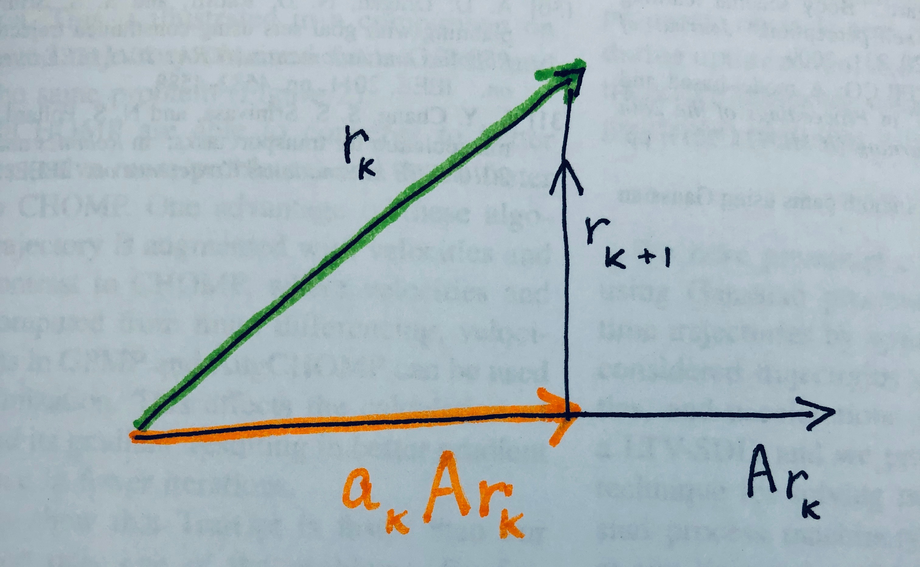
\[\begin{aligned} r_{k+1} &= b - Ax_{k+1} \\ &= b - A \Big(x_k + a_k(b-Ax_k) \Big) \\ &= (b - Ax_k) - a_kA(b-Ax_k) \\ &= r_k - a_kAr_k \end{aligned}\]Orthomin(1)
If you want to make the residue as small as possible, given some initial residue from some initial guess, then you want to minimize \(\|r_{k+1}\|\). Since \(aAr_k\) and \(r_k\) are simple vectors, we know how to minimize their difference: one should project \(r_k\) onto \(a_kAr_k\):
As shown in the tutorial on projection, projection of a vector \(x\) onto a vector \(y\) is given by \(P_y(x)= \frac{x^Ty}{y^Ty}y\). We wish to solve for the scalar knob \(a_k\), with \(x=r_k, y= Ar_k\):
\[\begin{aligned} a_k Ar_k &= \frac{ r_k^T (Ar_k) }{ (Ar_k)^T (Ar_k)} (Ar_k) \\ a_k &= \frac{ r_k^T (Ar_k) }{ (Ar_k)^T (Ar_k)} & \mbox{ remove multiplication by vector on both sides} \\ a_k &= \frac{\langle r_k, Ar_k \rangle}{\langle Ar_k, Ar_k \rangle} & \mbox{write as standard 2-inner products} \end{aligned}\]To minimize the 2-norm, we use standard 2-inner-product. This gives the Orthomin(1) method – from orthogonal projections. The purpose is to minimize the residual and the method seems to work for a general \(A\) matrix.
Steepest Descent
Now contrast Orthomin(1) with a second method, Steepest Descent. In Steepest Descent, you don’t have to choose the 2-norm to minimize the residual.
If \(A\) is Hermitian (can always diagonalize it, eigenvalues are real), and if it is positive definite (all eigenvalues are non-zero positive), then you can define another norm. This norm comes from the 2-norm, induced by \(A\):
\[\|x\|_A = \langle x, Ax \rangle^{1/2}\]When \(A\) is positive definite, it is truly a norm. We can use this norm instead.
In Steepest Descent, we will minimize the error \(e_k = x^{\star} - x_k\) instead of the residual \(r_k\). You might ask, how could you possibly compute the error if we don’t have access to \(x^{\star}\), which requires solving the problem? It turns out that terms cancel, so we don’t actually need to know \(x^{\star}\).
\[\begin{aligned} e_k &= x^{\star} - x_k \\ &= A^{-1}b - x_k \\ &= A^{-1}b + A^{-1}(r_k - b) & \mbox{since } r_k = b - Ax_k \implies A^{-1}(r_k -b) = - x_k \\ &= A^{-1}b - A^{-1}b + A^{-1}r_k \\ &= A^{-1}r_k \\ \end{aligned}\]We can now form a recurrence between \(e_{k+1}\) and \(e_{k}\):
\[\begin{aligned} e_{k} &= A^{-1}r_k & \mbox{as shown above} \\ e_{k+1} &= A^{-1} r_{k+1} & \mbox{consider the next time step} \\ e_{k+1} &= A^{-1} \Big( r_k - a_k A r_k \Big) \\ e_{k+1} &= A^{-1}r_k - a_k A^{-1}Ar_k \\ e_{k+1} &= A^{-1}r_k - a_k r_k & \mbox{because } A^{-1}A = I \\ e_{k+1} &= e_k - a_k r_k & \mbox{because } e_k = A^{-1}r_k \end{aligned}\]Our recurrence is between two vectors, \(e_k\) and a scaled \(r_k\). In order to minimize \(\|e_{k+1}\|_A\) given \(e_k\), we can simply project \(e_k\) onto \(r_k\).
We recall that the projection of a vector \(x\) onto a vector \(y\) is given by \(P_y(x) = \frac{x^Ty}{y^Ty}y\). Thus, we can compute the scaling \(a\) in \((ar_k)\) as:
\[a_k = \frac{\langle e_k, r_k \rangle_A}{\langle r_k, r_k \rangle_A} = \frac{\langle e_k, Ar_k\rangle }{\langle r_k, Ar_k\rangle } = \frac{\langle A^He_k, r_k\rangle }{\langle r_k, Ar_k\rangle } = \frac{\langle A e_k, r_k\rangle }{\langle r_k, Ar_k\rangle } = \frac{\langle r_k, r_k\rangle }{\langle r_k, Ar_k\rangle }\]We used the fact that \(A=A^H\) (since \(A\) is Hermitian) and the fact that \(e_k = A^{-1}r_k\), so \(Ae_k = r_k\). Note that now everything is expressed in terms of \(r_k\), not \(e_k\), since \(r_k\) is computable even when \(e_k\) isn’t. This method is called steepest descent and as we will see, it corresponds to a Krylov subspace method. Steepest descent requires that \(A=A^H\), and that \(A\) is positive definite for the norm definition.
Another Perspective on Steepest Descent
Another way to consider Steepest Descent is to consider that the algorithm at each step performs a gradient descent step with optimal step size. Consider the following objective function:
\[V(x) = x^HAx - 2b^Hx\]Then we can find the stationarity condition by finding the derivative and set to zero:
\[\begin{aligned} \nabla V = 2Ax - 2b = 0 \\ Ax = b \end{aligned}\]Our step is \(x_{k+1} = x_k - a_k \frac{1}{2}\nabla V(x_k)\)
At each step, we go as deep as you can, then we change to another direction.
Steepest Descent is a Krylov Subspace Method
Recall that a Krylov Subspace method builds solutions in the subpace
\[\mathcal{K}_k = \mbox{span} \{ \vec{b}, A \vec{b}, A^2 \vec{b}, \cdots \}\]In Steepest Descent, our iterative solutions are formed from the recurrence relation:
\[\vec{x}_{k+1} = \vec{x}_k + a_k( \vec{b} - A\vec{x}_k)\]One can prove via induction that Steepest Descent is a Krylov Subspace method. To show a brief example, suppose \(\vec{x}_0 = 0\). This implies
\[\begin{aligned} \vec{x}_1 &= x_0 + a_k (b-Ax_0) \\ \vec{x}_1 &= 0 + a_k (b-A \cdot 0) \\ \vec{x}_1 &= a_k b \\ \vec{x}_1 & \in \mbox{span} \{ \vec{b} \} \\ \end{aligned}\]Consider \(\vec{x}_2\).
\[\begin{aligned} \vec{x}_2 &= x_1 + a_k (b-Ax_1) \\ \vec{x}_2 &= (a_k b) + a_k \Big(b-A(a_k b)\Big) & \mbox{since } \vec{x}_1 &= a_k b \\ \vec{x}_2 &= a_kb + a_kb - a_k Aa_k b\\ \vec{x}_2 &= (2 a_k) b - (a_k^2) Ab \\ \vec{x_2} & \in \mbox{span} \Bigg\{ \vec{b}, A \vec{b} \Bigg\} \end{aligned}\]If you consider \(x_{k+1}\), it is not hard to show that if \(x_k\) was in a Krylov subspace, then so is \(x_{k+1}\). If \(x_0\) is non-zero, we simply start with a shifted \(\vec{b}\). As we recall, with an \(n\)-dimensional problem, we only need to do \(n\)-steps, then we span the whole space and are guaranteed to find the solution.
Orthomin(2)
We now seek an improvement on Orthomin(1). Orthomin(1) fails to converge if \(0\) is in the numerical range of \(A\). In Orthomin(1), we had a single orthogonality condition: \(r_{k+1} \perp A r_k\). Our step was in the direction of the residual \(r_k\). For the sake of generality, so we will call our descent direction \(p_k\), and for Orthomin(1), it just so happens that \(p_k = r_k\).
In Orthomin(2), we will now require two orthogonality conditions. We must be orthogonal to the previous two descent directions.
\[r_{k+1} \perp A p_k, Ap_{k-1}\]The question is, can we find some descent direction \(p_k\) such that we can accomplish this double orthogonality condition? As we showed previously, one of the orthogonality conditions is easy. If we want \(r_{k+1} \perp A p_k\), this is doable if we just pick a good scalar value \(a_k\). A slightly less trivial requirement is to have orthogonality to the previous descent direction.
Conjugate Gradients (CG)
Conjugate Gradients (CG) is a well-studied method introduced in 1952 by Hestenes and Stiefel [4] for solving a system of \(n\) equations, \(Ax=b\), where \(A\) is positive definite. Solving such a system becomes quite challenging when \(n\) is large. CG continues to be used today, especially in state-of-the-art reinforcement learning algorithms like TRPO.
The CG method is interesting because we never give a set of numbers for \(A\). In fact, we never form or even store the matrix \(A\). This could be desirable when \(A\) is huge. Instead, CG is simply a method for calculating \(A\) times a vector [1] that relies upon a deep result, the Cayley-Hamilton Theorem.
A common example where CG proves useful is minimization of the following quadratic form, where \(A \in \mathbf{R}^{n \times n}\):
\[f(x) = \frac{1}{2} x^TAx - b^Tx\]\(f(x)\) is a convex function when \(A\) is positive definite. The gradient of \(f\) is:
\[\nabla f(x) = Ax - b\]Setting the gradient equal to \(0\) allows us to find the solution to this system of equations, \(x^{\star} = A^{-1}b\). CG is an appropriate method to do so when inverting \(A\) directly is not feasible.
The CG Algorithm
We will maintain the square of the residual \(r\) at each step, which we call \(r_k\). If the square root of your residual is small enough, \(\sqrt{\rho_{k-1}}\), then you can quit. Your search direction is \(p\): the combination of your current r esidual and the previous search direction [2,3].
- \(x:=0\), \(r:=b\), \( \rho_0 := | r |^2 \)
- for \(k=1,\dots,N_{max}\)
- quit if \(\sqrt{\rho_{k-1}} \leq \epsilon \|b\|\)
- if \(k=1\)
- \( p:= r \)
- else
- \( p:= r + \frac{\rho_{k-1}}{\rho_{k-2}} \)
- \( w:=Ap \)
- \( \alpha := \frac{ \rho_{k-1} }{ p^Tw } \)
- \( x := x + \alpha p \)
- \( r := r - \alpha w \)
- \( \rho_k := |r|^2 \)
Along the way, we’ve created the Krylov sequence \(x\). Operations like \(x + \alpha p\) or \(r - \alpha w\) are \(\mathcal{O}(n)\) (BLAS level-1).
Properties of the Krylov Sequence It should be clear that \(x^{(k)}=p_k(A)b\), where \(p_k\) is a polynomial with degree \(p_k < k\), because \(x^{(k)} \in \mathcal{K}_k\). Surprisingly enough, the Krylov sequence is a two-term recurrence:
\[x^{(k+1)} = x^{(k)} + \alpha_k r^{(k)} + \beta_k (x^{(k)} - x^{(k+1)})\]for some values \(\alpha_k, \beta_k\).This means the current iterate is a linear combination of the previous two iterates. This is the basis of the CG algorithm.
The Art of Preconditioning
It turns out that CG will often just fail. The trick in CG is to change coordinates first (precondition) and then run CG on the system in the changed coordinates. This is because of round-off errors that accumulate, leading to unstability and divergence. For example, we may want to make the spectrum of \(A\) clustered.
Instead of solving a linear system \(Ax=b\), one can solve \(M^{-1}Ax = M^{-1}b\) for some carefully-chosen matrix \(M\). Theoretically, the problems are the same. Numerically, however, pre-conditioning is possibly advantageous. Preconditioning a matrix is an art. Here are two good criteria for which preconditioner should you use:
- Need \(M^{-1}y\) cheap to compute.
- We actually want \(M \approx A\). Then \(M^{-1}A \approx I\), and \(M^{-1}Ax = M^{-1}b\) is easy to solve.
Krylov subspaces and preconditioning can be combined. We basically need
\[x_k \in \mbox{span} \Bigg\{M^{-1}b, (M^{-1}A)M^{-1}b, \cdots, (M^{-1}A)^{k-1} M^{-1}b \Bigg\}\]That is our preconditioned Krylov subspace!
A good, generic preconditioner is a diagonal matrix, e.g.
\[M = \mbox{diag}(\frac{1}{A_{11}}, \dots, \frac{1}{A_{nn}})\]We will discuss pre-conditioning in more detail in an upcoming tutorial.
References
[1] Stephen Boyd. Conjugate Gradient Method. EE364b Lectures Slides, Stanford University. https://web.stanford.edu/class/ee364b/lectures/conj_grad_slides.pdf. Video.
[2] C.T. Kelley. Iterative Methods for Optimization. SIAM, 2000.
[3] C. Kelley. Iterative Methods for Linear and Nonlinear Equations. Frontiers in Applied Mathematics SIAM, (1995). https://archive.siam.org/books/textbooks/fr16_book.pdf.
[4] Magnus Hestenes and Eduard Stiefel. Method of Conjugate Gradients for Solving Linear Systems. Journal of Research of the National Bureau of Standards, Vol. 49, No. 6, December 1952. https://web.njit.edu/~jiang/math614/hestenes-stiefel.pdf.