Visual Odometry Tutorial

Visual Odometry (VO) is an important part of the SLAM problem. In this post, we’ll walk through the implementation and derivation from scratch on a real-world example from Argoverse. VO will allow us to recreate most of the ego-motion of a camera mounted on a robot – the relative translation (but only up to an unknown scale) and the relative rotation.

Table of Contents:

• Data: a sequence from Argoverse
• Moving to the camera coordinate frame
• Starting out with VO: manually annotating correspondences
• Fitting Epipolar Geometry
• Recovering the relative motion
• Digging in to Epipolar Geometry Conventions
• Using SIFT to Generate Correspondences

Data: a sequence from Argoverse

Argoverse is a large-scale public self-driving dataset [1]. We’ll use two images from the front-center ring camera of the 273c1883-673a-36bf-b124-88311b1a80be vehicle log. The log can be downloaded here as part of the train1 subset of vehicle logs. These images are captured at 1920 x 1200 px resolution @30 fps, but a preview of the log @15 fps and 320p is shown below (left). Below on the right, we show the egovehicle’s trajectory in the global frame (i.e. city coordinate frame) which we wish to reconstruct from 2d correspondences. The evolution of the trajectory is shown from red to green: first we drive straight, then turn right. Two dots are shown, the first in magenta, and the second in cyan (light blue). These are the poses when the two images we’ll focus on were captured.

Consider the coordinate system conventions of Argoverse (shown below)

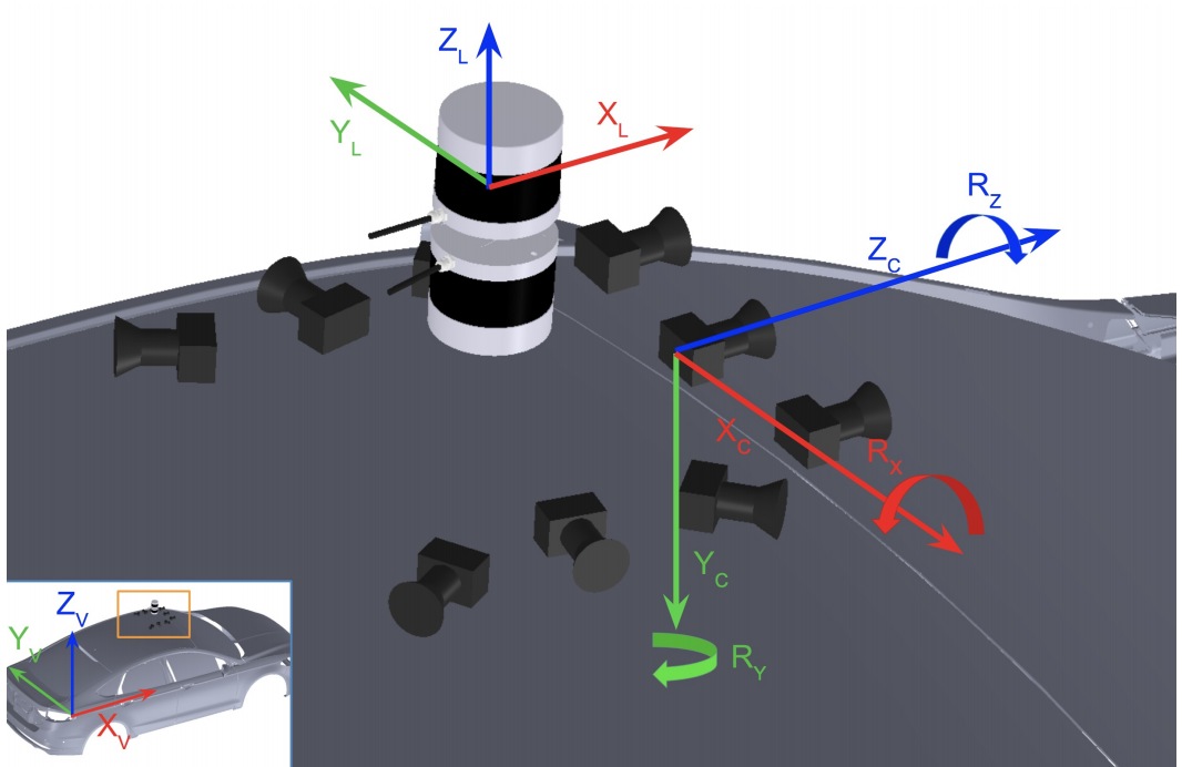
The positive x-axis extends in the forward driving direction, and +y points left out of the car when facing forward. The z-axis points upwards, opposite to gravity. With a quick glance at the trajectory above (right), we see the change in pose between the two locations of interest is to rotate the egovehicle coordinate right by about 30 degrees, and then to translate forward by about 12 meters in the +x direction. We’ll now measure this exactly:

from argoverse.data_loading.pose_loader import get_city_SE3_egovehicle_at_sensor_t

ts1 = 315975640448534784 # nano-second timestamp
ts2 = 315975643412234000

log_id = '273c1883-673a-36bf-b124-88311b1a80be'
dataset_dir = '/Users/johnlambert/Downloads/visual-odometry-tutorial/train1'

city_SE3_egot1 = get_city_SE3_egovehicle_at_sensor_t(ts1, dataset_dir, log_id) 
city_SE3_egot2 = get_city_SE3_egovehicle_at_sensor_t(ts2, dataset_dir, log_id) 

t1 = city_SE3_egot1.translation
t2 = city_SE3_egot2.translation
print(t1) # prints array([-274.0, 3040.1,  -19.0])
print(t2) # prints array([-273.2, 3052.5,  -19.1])

Sure enough, we see that the second pose is about +12 meters further along the y-axis of the city coordinate system than the first pose. Now, we need to determine the relative orientation.

When we consider an SE(3) transformation i1_T_i2, it represents the transformation that brings points and rays from coordinate system i2 to coordinate system i1. It also represents i2’s pose inside i1’s frame. Also given for free by i1_T_i2 is the rotation and translation to move one coordinate frame i1 to the other’s (i2) position and orientation.

If we want to move the pink point (shown on right), lying at (4,0,0) in i2’s coordinate frame, and place it into i1’s coordinate frame, we can see the steps below . Rotate the point by -32 degrees, then translate it by +12 meters along x, and translate -2 meters along y. This is also the same process we would use to move i1’s frame to i2’s frame, if we fix the Cartesian grid in the background and consider the frame as a set of lines (i.e. points) moving from living in i2’s frame to living in i1’s frame.

Here, i1 represents the egovehicle frame @t=1, i.e. egot1, and i2 represents the egovehicle frame @t=2, i.e. egot2. Let city_SE3_egot1 be the SE(3) transformation that takes a point in egot1’s frame, and moves it into the city coordinate frame. Then:

egot1_SE3_city = city_SE3_egot1.inverse()
egot1_SE3_egot2 = egot1_SE3_city.compose(city_SE3_egot2)

As discussed previously, egot1_SE3_egot2 is composed of the (R,t) that (A) bring points living in 2’s frame into 1’s frame and (B) is the pose of the egovehicle @t=2 when it is living in egot1’s frame, and (C) rotates 1’s frame to 2’s frame. Thus, the relative rotation and translation below are what we hope to use VO to re-accomplish.

from scipy.spatial.transform import Rotation

egot1_R_egot2 = egot1_SE3_egot2.rotation
egot1_t_egot2 = egot1_SE3_egot2.translation

r = Rotation.from_matrix(egot1_R_egot2)
print(r.as_euler('zyx', degrees=True)) # prints [-32.47   0.587  -0.436 ]
print(np.round(egot1_t_egot2,2)) # prints [12.27 -1.88  0.  ]

It should be clear now that the relative yaw angle is -32 degrees (about z-axis), and roll and pitch are minimal (<1 degree), since the ground is largely planar.

Moving to the camera coordinate frame

There is an important shift we need to make before proceeding to the VO section – we need to switch to the camera coordinate frame. In the camera coordinate frame, the +z-axis points out of the camera, and the y-axis is now the vertical axis. Since this is the front-center camera, the car is now moving in the +z direction, and we’ll express our yaw about the y-axis.

However, since +y now points into the ground (with the gravity direction), and by the right hand rule, our rotation should swap sign.

We’ll load the camera extrinsics from disk. There are multiple possible conventions, but we’ll define our extrinsics as the SE(3) object that bring points from one frame (in our case, the egovehicle frame) into the camera frame, camera_T_egovehicle:

from argoverse.utils.calibration import load_calib

calib_fpath = '/Users/johnlambert/Downloads/visual-odometry-tutorial/train1/273c1883-673a-36bf-b124-88311b1a80be/vehicle_calibration_info.json'
calib_dict = load_calib(calib_fpath)
camera_T_egovehicle = calib_dict['ring_front_center'].extrinsic
camera_T_egovehicle = SE3(rotation=camera_T_egovehicle[:3,:3], translation=camera_T_egovehicle[:3,3])

We’ll now compose poses to obtain the relative rotation and translation from the camera frame @t=1 cam1, to the camera frame @t=2 cam2:

egovehicle_T_camera = camera_T_egovehicle.inverse()

city_SE3_cam1 = city_SE3_egot1.compose(egovehicle_T_camera)
city_SE3_cam2 = city_SE3_egot2.compose(egovehicle_T_camera)

cam1_SE3_city = city_SE3_cam1.inverse()
cam1_SE3_cam2 = cam1_SE3_city.compose(city_SE3_cam2)

cam1_R_cam2 = cam1_SE3_cam2.rotation
cam1_t_cam2 = cam1_SE3_cam2.translation

r = Rotation.from_matrix(cam1_R_cam2)
print('Ground truth relative rotation: ', r.as_euler('zyx', degrees=True))
### prints [-0.37137223 32.4745113  -0.42247361]

We can see that they yaw angle is now 32.47 degrees around the y-axis, i.e. the sign is flipped, as expected. If we look at the relative translation, we see we move mostly in the +z direction, but slightly in +x as well:

import numpy as np
print('Recover t=', cam1_t_cam2) ## prints [ 2.63 -0.029  12.05] 
cam1_t_cam2 /= np.linalg.norm(cam1_t_cam2)
print('Up to a scale ', cam1_t_cam2) # [ 0.21  -0.0024  0.976]

Now we’ll recover these measurements from 2d correspondences and intrinsics.

Starting out with VO: manually annotating correspondences

First, to get VO to work, we need accurate 2d keypoint correspondences between a pair of images. These can be estimated with classic (e.g. DoG+SIFT+RANSAC) or deep methods (e.g. SuperPoint+SuperGlue), but for the sake of this example, we’ll ensure completely accurate correspondences using an a simple 200-line interactive Python script [code here]. that uses matplotlib’s ginput() to allow a user to manually click on points in each image and cache the correspondences to a pickle file.

# within the visual-odometry-tutorial/ directory
export IMG_DIR=train1/273c1883-673a-36bf-b124-88311b1a80be/ring_front_center
python collect_ground_truth_corr.py --img_fpath1 ${IMG_DIR}/ring_front_center_315975640448534784.jpg --img_fpath2 ${IMG_DIR}/ring_front_center_315975643412234000.jpg --experiment_name argoverse_2_E_1.pkl

However, since humans are not perfect “clickers”, there will be measurement error. Therefore, we’ll need to manually provide more than the minimal number of correspondences to account for noise (recall that is 5 for an Essential matrix, and 8 for a Fundamental matrix).

Below we show the first image (left) and then later image (right) as the egovehicle drives forward and then starts to make a right turn. While there are dynamic objects in the scene (particularly the white vehicles visible in the left image), much of the scene is static (signs, walls, streetlights, parked cars), which we’ll capitalize on.

Fitting Epipolar Geometry

We now need to fit the epipolar geometry relationship. First, we’ll load the keypoint correspondences that we annotated from disk:

import pickle
pkl_fpath = f'/Users/johnlambert/Downloads/visual-odometry-tutorial/labeled_correspondences/argoverse_2_E_1.pkl'
with open(str(pkl_fpath), 'rb') as f:
	d = pickle.load(f)
X1 = np.array(d['x1'])
Y1 = np.array(d['y1'])
X2 = np.array(d['x2'])
Y2 = np.array(d['y2'])

We’ll form two Nx2 arrays to represent the correspondences of 2d points to other 2d points:

img1_kpts = np.hstack([ X1.reshape(-1,1), Y1.reshape(-1,1) ]).astype(np.int32)
img2_kpts = np.hstack([ X2.reshape(-1,1), Y2.reshape(-1,1) ]).astype(np.int32)

We’ll let OpenCV handle the linear system solving and SVD computation, so we just need a few lines of code. We already know the camera intrinsics, so we prefer to fit the Essential matrix. As we recall, the F matrix can be obtained from the E matrix as:

def get_fmat_from_emat(i2_E_i1: np.ndarray, K1: np.ndarray, K2: np.ndarray) -> np.ndarray:
	""" """
	i2_F_i1 = np.linalg.inv(K2).T @ i2_E_i1 @ np.linalg.inv(K1)
	return i2_F_i1

We fit the Essential matrix with the 5-Point Algorithm [2], and plot the epipolar lines:

import cv2
K = calib_dict['ring_front_center'].K[:3,:3]
cam2_E_cam1, inlier_mask = cv2.findEssentialMat(img1_kpts, img2_kpts, K, method=cv2.RANSAC, threshold=0.1)
print('Num inliers: ', inlier_mask.sum()) ### prints "Num inliers: 8"
cam2_F_cam1 = get_fmat_from_emat(cam2_E_cam1, K1=K, K2=K)
draw_epilines(img1_kpts, img2_kpts, img1, img2, cam2_F_cam1)

Only 8 of our 20 annotated correspondences actually fit the model, but this may be OK. To make sure the fit is decent, we can compare epipolar lines visually.

Epipolar Lines As you may know, a point in one image is associated with a 1d line in the other. Furthermore, epipolar lines converge at an epipole. Note the location of the epipole in the left image – it is precisely where the front-center camera was located when the second image (right) is captured. We use one color for each correspondence, and indeed all points seem to lie along their epipolar lines. This is great.

Recovering the relative motion

It’s now time to finally recover the relative motion from the Essential matrix. We’ll use OpenCV’s implementation of the latter portion of the 5-Point Algorithm [2], which verifies possible pose hypotheses by checking the cheirality of each 3d point. 2d points are lifted to 3d by triangulating their 3d position from two views. The cheirality check means that the triangulated 3D points should have positive depth.

_num_inlier, cam2_R_cam1, cam2_t_cam1, _ = cv2.recoverPose(cam2_E_cam1, img1_kpts, img2_kpts, mask=inlier_mask)
r = Rotation.from_matrix(cam2_R_cam1)
print(r.as_euler('zyx', degrees=True)) ### prints [  0.681 -33.107   0.755]
print(np.round(cam2_t_cam1, 2)) ## prints "array([ 0.36,  0.01, -0.93])"

We have a problem, though. The relative rotation here is not +32 degrees as expected, but rather -33 degrees. The translation is in the -z direction, rather than +0.98 in the +z direction. The reason is that we recovered the inverse.

Digging in to Epipolar Geometry Conventions

Consider why this occurred – given point correspondences \(\{(\mathbf{x}_0,\mathbf{x}_1)\}\) respectively from two images \(I_0\), \(I_1\), and camera intrinsics \(K\), OpenCV solves for an Essential matrix \({}^1 E_0\):

Where does this equation come from? Consider the following camera setup from Szeliski (p. 704) [3]:

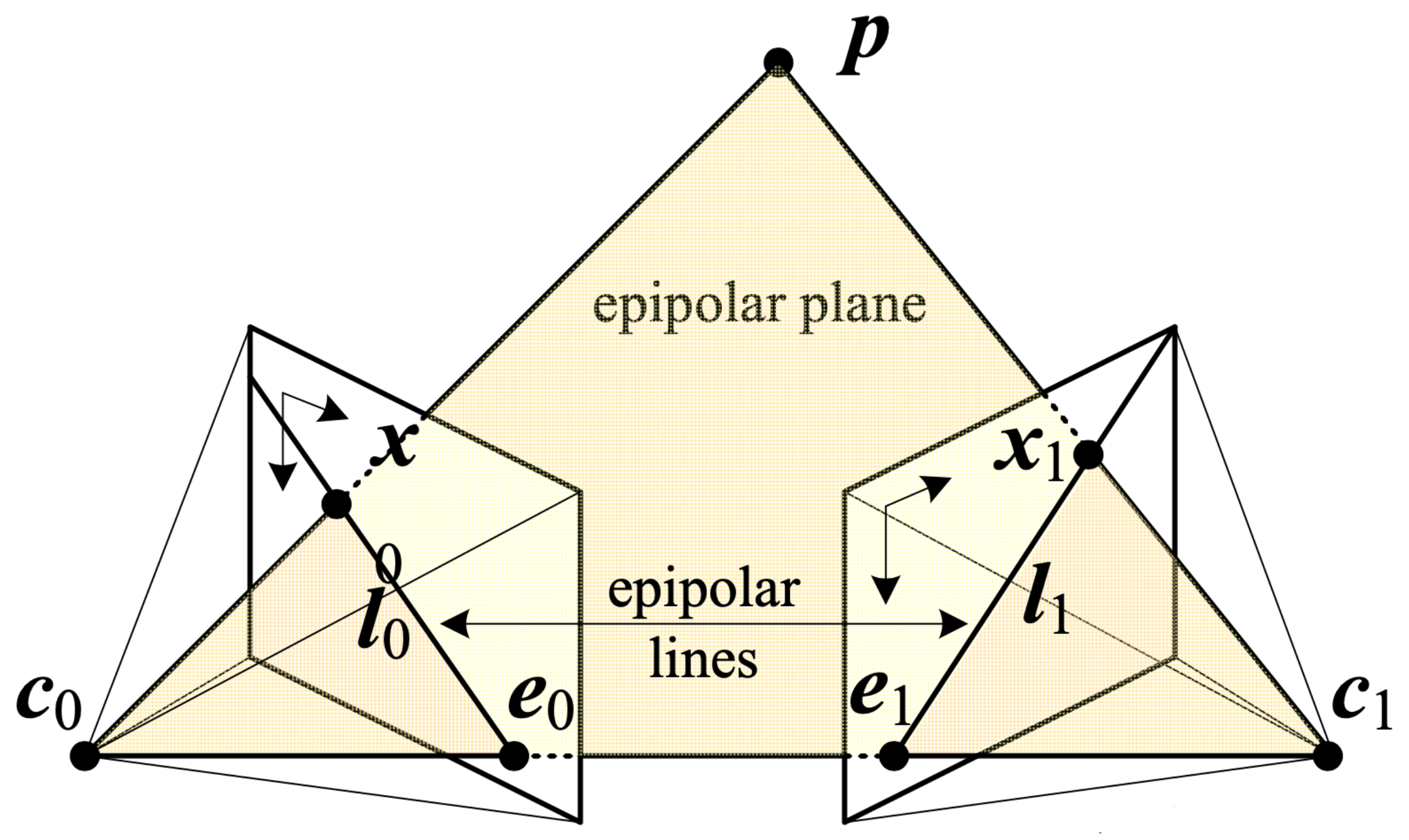
Szeliski shows that a 3D point \(\mathbf{p}\) being viewed from two cameras can be modeled as:

where \(\hat{\mathbf{x}}_j = \mathbf{K}_j^{-1} \mathbf{x}_j\) are the (local) ray direction vectors. Note that \({}^1\mathbf{R}_0\) and \({}^1\mathbf{t}_0\) define an SE(3) 1_T_0 object that transforms \(\mathbf{p}_0\) from camera 0’s frame to camera 1’s frame. We’ll refer to these just as \(\mathbf{R}\) and \(\mathbf{t}\) for brevity in the following derivation.

We can eliminate the \(+ \mathbf{t}\) term by a cross-product. This can be achieved by multiplying with a skew-symmetric matrix as \([\mathbf{t}]_{\times} \mathbf{t} = 0\). Then:

Swapping sides and taking the dot product of both sides with \(\hat{\mathbf{x}}_1\) yields

Since the cross product \([\mathbf{t}]_x\) returns 0 when pre- and post-multiplied by the same vector, we arrive at the familiar epipolar constraint, where \(\mathbf{E}= [\mathbf{t}]_{\times} \mathbf{R}\):

If we assemble the SE(3) object 1_T_0 \(({}^1\mathbf{R}_0, {}^1\mathbf{t}_0)\) from the decomposed E matrix, and then invert the pose to get 0_T_1, i.e. camera 1’s pose inside camera 0’s frame, we find everything is as expected:

import numpy as np
from argoverse.utils.se3 import SE3

cam2_SE3_cam1 = SE3(cam2_R_cam1, cam2_t_cam1.squeeze() )
cam1_SE3_cam2 = cam2_SE3_cam1.inverse()
cam1_R_cam2 = cam1_SE3_cam2.rotation
cam1_t_cam2 = cam1_SE3_cam2.translation

r = Rotation.from_matrix(cam1_R_cam2)
print(r.as_euler('zyx', degrees=True)) ## prints "[-0.32  33.11 -0.45]"
print(np.round(cam1_t_cam2,2)) ## [0.21 0.   0.98]

As we recall, the ground truth relative rotation cam1_R_cam2 could be decomposed into z,y,x Euler angles as [-0.37 32.47 -0.42]. The relative translation cam1_t_cam2 could be recovered up to a scale as [ 0.21 -0.0024 0.976]. Our error is less than one degree in each Euler angle, and the translation direction is perfect at least to two decimal places.

Using SIFT to Generate Correspondences

Of course we can’t annotate correspondences in real-time nor would we want to do so in the real-world, so we’ll turn to algorithms to generator keypoint detections and descriptors. Since its 20-year patent has expired, SIFT now ships out of the box with OpenCV:

import cv2
opencv_obj = cv2.SIFT_create()
cv_keypoints, descriptors = opencv_obj.detectAndCompute(gray_img, None)

What sort of keypoints does SIFT effectively capitalize on? Surprisingly, it can make use of vegetation, curbs, in addition to the parked cars and painted text and artwork on the walls we used earlier. While there are a few noisy correspondences, most of the “verified” correspondences look quite good:

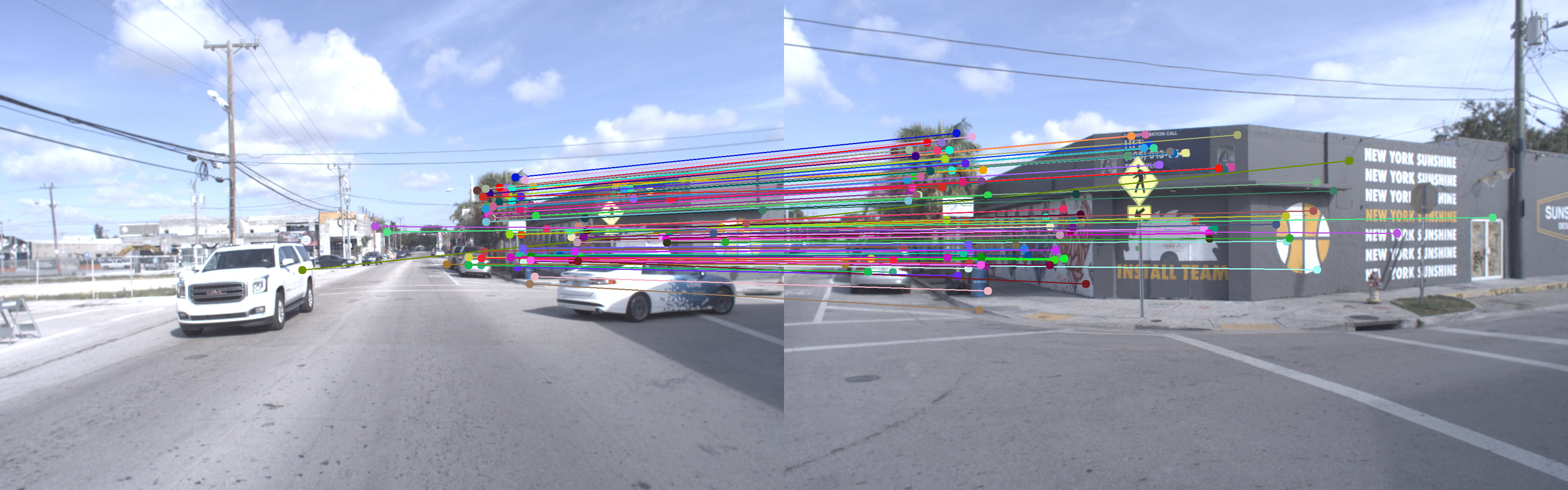
The pose error is slightly higher with SIFT than our manually-annotated correspondences: first, our estimated Euler rotation angles are now up to \(1.4^{\circ}\) off. Using SIFT correspondences, the 5-Point Algorithm predicts [ 0.71, 32.56, -1.74] vs. ground truth angles of [-0.37, 32.47, -0.42] degrees. While the estimated rotation is very close about the y-axis (just \(0.1^\circ\) off), the rotation about the z-axis is now about \(1.3^\circ\) off and \(1.0^\circ\) off about the x-axis.

What about the error on the translation direction? Using these SIFT correspondences, our estimated unit translation i1ti2 = [ 0.22, -0.027, 0.97], vs. ground truth of [ 0.21 , -0.0024, 0.976 ]. This looks decent, and we can compute the actual amount of error in degrees using the cosine formula for dot products:

import numpy as np
norm1 = np.linalg.norm(gt_i1ti2)
norm2 = np.linalg.norm(i1ti2)
err_rad = np.arccos( gt_i1ti2.dot(i1ti2) / (norm1 * norm2) )
np.rad2deg(err_rad) # prints 1.68177

As shown above, the angular error between estimated and ground truth translation vectors comes out to about \(1.68^\circ\).

Our visual odometry is complete. You can find the full code to reproduce this here.

import glob
from pathlib import Path
from typing import List

import cv2
import matplotlib.pyplot as plt
import numpy as np
from colour import Color
from scipy.spatial.transform import Rotation

from utils import get_matches, load_image

from ransac import ransac_fundamental_matrix


DATA_ROOT = Path(__file__).resolve().parent.parent / "data"


def get_emat_from_fmat(i2_F_i1: np.ndarray, K1: np.ndarray, K2: np.ndarray) -> np.ndarray:
    """ Create essential matrix from camera instrinsics and fundamental matrix"""
    i2_E_i1 = K2.T @ i2_F_i1 @ K1
    return i2_E_i1


def load_log_front_center_intrinsics() -> np.array:
    """Provide camera parameters for front-center camera for Argoverse vehicle log ID:
    273c1883-673a-36bf-b124-88311b1a80be
    """
    fx = 1392.1069298937407  # also fy
    px = 980.1759848618066
    py = 604.3534182680304

    K = np.array([[fx, 0, px], [0, fx, py], [0, 0, 1]])
    return K


def get_visual_odometry():
    """ """
    img_wildcard = f"{DATA_ROOT}/vo_seq_argoverse_273c1883/ring_front_center/*.jpg"
    img_fpaths = glob.glob(img_wildcard)
    img_fpaths.sort()
    num_imgs = len(img_fpaths)

    K = load_log_front_center_intrinsics()

    poses_wTi = []

    poses_wTi += [np.eye(4)]

    for i in range(num_imgs - 1):
        img_i1 = load_image(img_fpaths[i])
        img_i2 = load_image(img_fpaths[i + 1])
        pts_a, pts_b = get_matches(img_i1, img_i2, n_feat=int(4e3))

        # between camera at t=i and t=i+1
        i2_F_i1, inliers_a, inliers_b = ransac_fundamental_matrix(pts_a, pts_b)
        i2_E_i1 = get_emat_from_fmat(i2_F_i1, K1=K, K2=K)
        _num_inlier, i2Ri1, i2ti1, _ = cv2.recoverPose(i2_E_i1, inliers_a, inliers_b)

        # form SE(3) transformation
        i2Ti1 = np.eye(4)
        i2Ti1[:3, :3] = i2Ri1
        i2Ti1[:3, 3] = i2ti1.squeeze()

        # use previous world frame pose, to place this camera in world frame
        # assume 1 meter translation for unknown scale (gauge ambiguity)
        wTi1 = poses_wTi[-1]
        i1Ti2 = np.linalg.inv(i2Ti1)
        wTi2 = wTi1 @ i1Ti2
        poses_wTi += [wTi2]

        r = Rotation.from_matrix(i2Ri1.T)
        rz, ry, rx = r.as_euler("zyx", degrees=True)
        print(f"Rotation about y-axis from frame {i} -> {i+1}: {ry:.2f} degrees")

    return poses_wTi


def plot_poses(poses_wTi: List[np.ndarray], figsize=(7, 8)) -> None:
    """
    Poses are wTi (in world frame, which is defined as 0th camera frame)
    """
    axis_length = 0.5

    num_poses = len(poses_wTi)
    colors_arr = np.array([[color_obj.rgb] for color_obj in Color("red").range_to(Color("green"), num_poses)]).squeeze()

    _, ax = plt.subplots(figsize=figsize)

    for i, wTi in enumerate(poses_wTi):
        wti = wTi[:3, 3]

        # assume ground plane is xz plane in camera coordinate frame
        # 3d points in +x and +z axis directions, in homogeneous coordinates
        posx = wTi @ np.array([axis_length, 0, 0, 1]).reshape(4, 1)
        posz = wTi @ np.array([0, 0, axis_length, 1]).reshape(4, 1)

        ax.plot([wti[0], posx[0]], [wti[2], posx[2]], "b", zorder=1)
        ax.plot([wti[0], posz[0]], [wti[2], posz[2]], "k", zorder=1)

        ax.scatter(wti[0], wti[2], 40, marker=".", color=colors_arr[i], zorder=2)

    plt.axis("equal")
    plt.title("Egovehicle trajectory")
    plt.xlabel("x camera coordinate (of camera frame 0)")
    plt.ylabel("z camera coordinate (of camera frame 0)")


# if __name__ == '__main__':
#   get_visual_odometry()

References

1. Ming-Fang Chang, John Lambert, Patsorn Sangkloy, Jagjeet Singh, Slawomir Bak, Andrew Hartnett, De Wang, Peter Carr, Simon Lucey, Deva Ramanan, James Hays. Argoverse: 3D Tracking and Forecasting with Rich Maps. CVPR 2019.

2. David Nistér. An efficient solution to the five-point relative pose problem. Pattern Analysis and Machine Intelligence, IEEE Transactions on, 26(6):756–770, 2004.

3. Richard Szeliski. Computer Vision: Algorithms and Applications, 2nd Edition. 2022.