Linear Algebra Without the Agonizing Pain

Table of Contents:

• Null Space
• Column Space
• Projection of a Vector onto a Vector
• Gram-Schmidt
• Solving Systems of Equations
• Singular Value Theorem (SVD)
• Computation of the SVD
• Sherman-Morrison
• Sherman-Woodbury-Woodbury Formula

Linear Algebra Definitions

Before we do anything interesting with machine learning or optimization, we’ll need to review some absolutely essential linear algebra concepts.

Suppose we have two vectors \(u,v \in \mathbf{R}^{n \times 1}\). Their outer product is defined as \(u \cdot v^T\), which is an \(n \times n\) matrix. The inner product of \(u\) and \(v\) is defined \(u^Tv \in \mathbf{R}^{1 \times 1}\), a scalar.

Orthogonal vectors satisfy \(v^Tu = 0\). For all \(x \neq 0\), if the quadratic form is positive \(x^TAx > 0\), then the matrix is symmetric positive matrix; if instead \(x^TAx \geq 0\), the matrix is symmetric positive semi-definite.

A vector norm assigns a scalar value to vector or matrix. It turns out that all norms are equivalent, meaning we can bound a certain norm above and below

e.g. \(\|x\|_{\alpha} \leq C_{\alpha \beta} \| x \|_{\beta}\), or \(\|x\|_2 \leq \|x\|_1 \leq \sqrt{n} \|x\|_2\).

Many matrix norms are induced from vector norms.

Matrix Rank

Vector Space

Null Space of a Matrix

Given \(A \in \mathbb{R}^{m \times n}\), the null space of \(A\) is the set of vectors which are sent to the zero vector:

Multiplication by \(A\) can be seen as a function which sends a vector \(x \in \mathbb{R}^n\) to a vector \(Ax \in \mathbb{R}^m\).

Of course, \(\mathcal{N}(A)\) always contains the zero vector, i.e. \({0} \in \mathcal{N}(A)\). But the question is, does it contain any other vectors? If the columns of \(A\) are linearly independent, then we can always say \(\mathcal{N}(A) = {0} \).

Column Space (Range) of a Matrix

Given an \(m \times n\) matrix \(A\), we would like to know for which vectors \(b \in \mathbb{R}^m\) the system \(Ax = b\) has a solution. Let’s define the columns of \(A\) as:

The column space of \(A\) is

The system \(Ax = b\) has a solution if and only if \(b \in C(A)\), equivalent to stating \(b\) is in the range of \(A\): \(b \in R(A)\).

Rank-Nullity Theorem

Let \(A\) be any matrix such that \(A \in \mathbb{R}^{m \times n}\).

Orthogonal Complement

Matrix Calculus

Two identities are essential: gradients of matrix-vector products and of quadratic forms.

• \( \nabla_x (Ax) = A^T\)
• \(\nabla_x (x^TAx) = Ax + A^Tx\)

When \(A\) is symmetric, which is often the case, \(A = A^T\) and thus \(\nabla_x (x^TAx) = 2Ax \)

John Duchi explains exactly why identies are true in [1].

Projection of a Vector onto a Vector

We’ll now derive the basic formulas that wil allow us to compute an orthonormal basis, via Gram Schmidt, which relies upon projection of vectors onto other vectors.

Cosine Rule

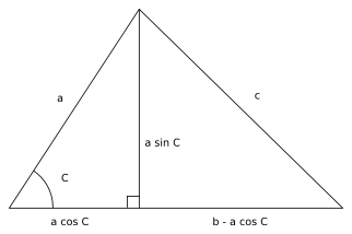
First, we need to derive the Cosine Rule. Consider the following triangle, which can be divided into two right triangles by drawing a line that passes through point \(B\) and is perpendicular to side \(b\).

Consider the right subtriangle, which is a “right triangle” with edge length \(c\) as its hypotenuse. By the Pythagorean Theorem,

Dot Product as a Cosine

Consider two arbitrary vectors \(A\) and \(B\). We can form a triangle with these two sides and a third side connecting the ends of \(A\) and \(B\). We let \(\theta\) be the angle between \(A\) and \(B\).

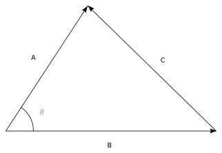
We showed above via the Law of Cosines that \(C \cdot C = \|A\| + \|B\| - 2 \|A\| \|B\| \mbox{ cos }(\theta)\) , thus

Projection by Inner Products

Consider two vectors \(x,y \in \mathbb{R}^n\). We write their “inner product” as

The “norm” of a vector \(x\), a measure of its length, is computed as

By trigonometry, we see a triangle:

We know that the vector \(\vec{e}_y = \frac{y}{||y||}\). The projection of \(x\) onto the vector \(y\), denoted as \(P_y(x)\), is equivalent to computing \( cos(\theta) = \frac{adj}{hyp} \), where the adjacent side of the triangle is the vector \(\vec{y}\) and the hypotenuse is the vector \(\vec{x}\). We can reformulate this equation as

In our case, this becomes

We recognize this as part of the cosine rule for dot products. Plugging this expression into the cosine rule, we see:

We can easily write out the projection at this point, as merely the computation of the vector \(X_y\). We have obtained a closed form expression above for its length, and multiplying it by the unit vector in the direction of \(\vec{y}\), we see:

where \(\frac{x^Ty}{||y||^2}\) is just a scalar coefficient.

The Gram-Schmidt Procedure

Suppose we have a set of \(k\) vectors \(\{a_1, \dots, a_k\}\) such that \(a_i \in \mathbb{R}^n\) are all independent. The objective of the Gram Schmidt procedure is to produce an orthonormal set of vectors \(\{ q_1, \dots, q_k \}\) such that \(q_i \in \mathbb{R}^n\). We can do so by iteratively subtracting the portion of the next vector \(a_{i+1}\) that projects onto \(a_i\). For example, to find a vector which is orthogonal to the first, we could compute

To find many vectors, we can follow an iterative procedure:

Gram Schmidt: Suppose we start with the red and blue vectors. We wish to obtain two orthogonal, unit length vectors (green and magenta).

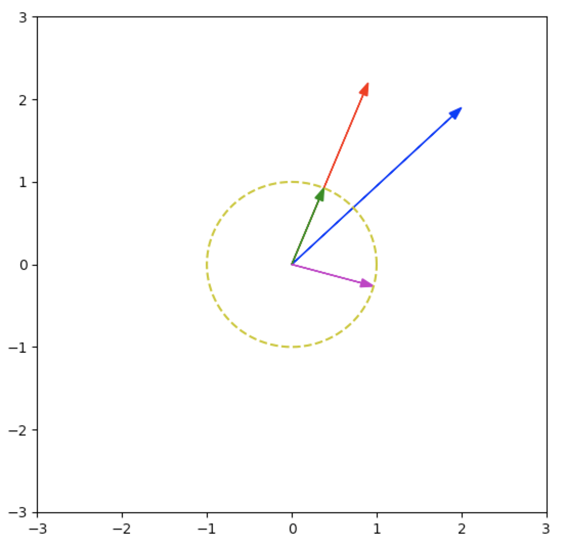
In a few lines of Python, we can generate this plot:

import numpy as np
import matplotlib.pyplot as plt

def plot_2d_vector(v: np.ndarray, c: str) -> None:
    """Plot a 2d vector as an arrow."""
    plt.arrow(0, 0, v[0], v[1], color=c, head_width=.1, length_includes_head=True)

def plot_circle_points() -> None:
    """Generates n points along a circle's perimeter."""
    n = 100
    radius = 1
    circ_x = np.array([np.cos(2*np.pi/n*x)*radius for x in range(0,n+1)])
    circ_y = np.array([np.sin(2*np.pi/n*x)*radius for x in range(0,n+1)])
    plt.plot(circ_x,circ_y, 'y--')

def plot_unit_circle_gs() -> None:
    a1 = np.array([0.9,2.2])
    a2 = np.array([2.,1.9])
    plot_2d_vectors(a1,a2,'r','b')

    # `q1` is just normalized `a1`.
    q1 = a1 / np.linalg.norm(a1)

    # Subtracts the projection of `a2` onto `q1`, from `a2`.
    q2_tilde = a2 - (a2.T.dot(q1)) * (q1)
    q2 = q2_tilde / np.linalg.norm(q2_tilde)

    plot_2d_vector(q1, 'g')
    plot_2d_vector(q2, 'm')
    plot_circle_points()
    plt.xlim([-3,3])
    plt.ylim([-3,3])
    plt.show()

A simple implementation of classical Gram-Schmidt (CGS) algorithm can be found here. We create \(n\) orthonormal vectors \(q_k\):

from typing import Tuple
import numpy as np

def classical_gs(A: np.ndarray) -> Tuple[np.ndarray, np.ndarray]:
    """Compute QR decomposition using Classical Gram Schmidt (MGS).

    Args:
        A: Numpy array of shape (m,n). (Must be full rank).

    Returns:
        Q: Orthogonal matrix of shape (m,n).
        R: Square Upper triangular matrix of shape (n,n).
    """
    m,n = A.shape
    Q = np.zeros((m,m))
    R = np.zeros((n,n))
    for k in range(n):
        for i in range(k):
            R[i,k] = Q[:,i].T.dot(A[:,k])
            A[:,k] -= R[i,k] * Q[:,i]
        R[k,k] = np.linalg.norm(A[:,k])
        Q[:,k] = A[:,k] / R[k,k]

    return Q, R

Solving Systems of Equations

Overdetermined Systems

Here, matrix \(A\) is a skinny, full-rank matrix. We cannot solve such a system, so instead we minimize a residual \(r\), i.e. we minimize \(\lVert r \rVert^2 = \lVert Ax-y \rVert^2\). We find an approximate solution to \(Y=Ax\).

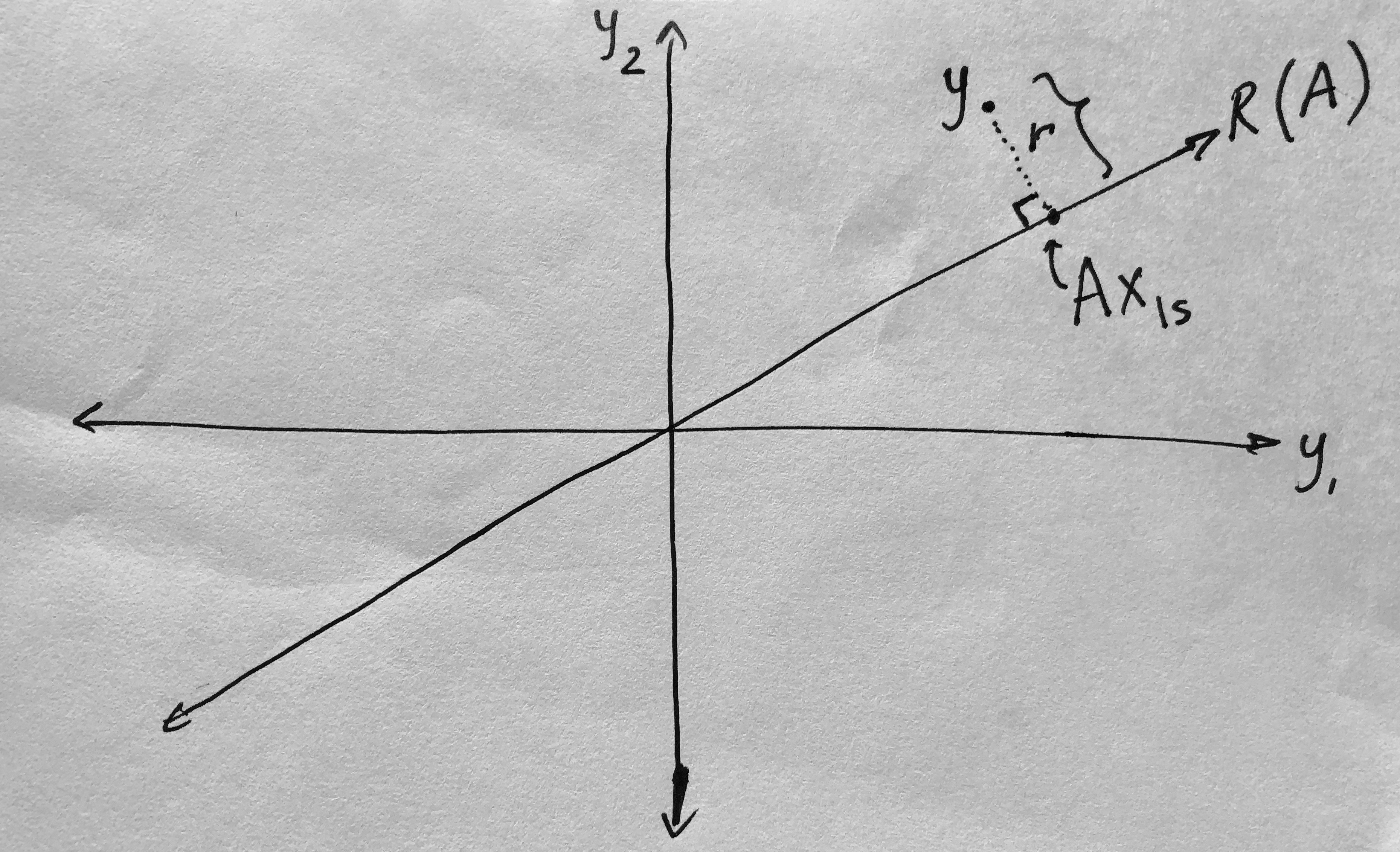
Formally, we minimize some objective function \(J\):

We can set its gradient to zero, and since the objective is the square of an affine function, it is convex, so we can find its true, global minimum:

Multiply on the left by \((A^TA)^{-1}\), and we recover the least squares solution:

We are projecting \(y\) onto the the range of \(A\):

We call \(A^{\dagger}\) a left-inverse of \(A\) because \(A^{\dagger}A=I\).

Underdetermined Systems

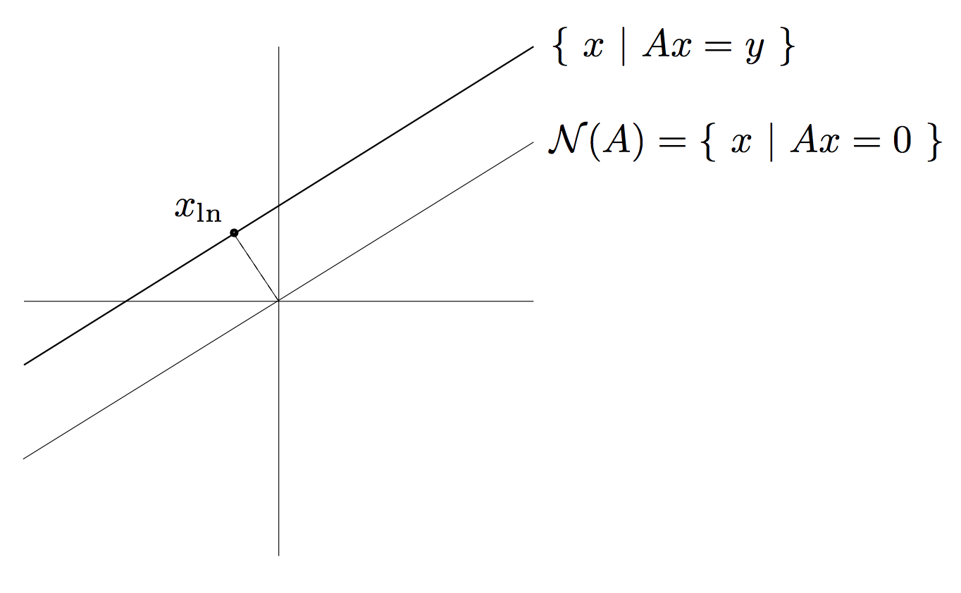
Here \(A\) is a fat, full-rank matrix. We can always solve such a system, and there will be an infinite # of solutions.

We often choose to find the smallest solution, i.e. the one closest to the origin

Source: [3]

We call this a least-norm (\(x_{ln}\) ) solution, because we minimize \(\lVert x \rVert\):

By introducing Lagrange multipliers, we find

We have two optimality conditions:

From condition (1), we see that

Substituting this into condition (2), we observe:

We call \(A^{\dagger}\) a right-inverse of \(A\) because \(AA^{\dagger}=I\).

Singular Value Decomposition (SVD)

The Singular Value Decomposition (SVD), although often attributed to Eckart and Young, was discovered in the late 19th century by Beltrami, Jordan, Sylvester. The SVD is a type of factorization, also known as a decomposition in numerical linear algebra. While some factorizations exist for all matrices, exist for only certain matrices. The SVD works for any matrix, even those that are nonsquare or include complex elements.

SVD Definition

Formally, any matrix (complex or real) \(A \in C^{m \times n}\) can be decomposed into \(A=U \Sigma V^T\) where \(U \in \mathbf{C}^{m \times m}, V \in \mathbf{C}^{n \times n}\).

where \(U\), \(V\) are orthogonal matrices, meaning \(U^TU = I\), \(UU^T=I\), and \(\Sigma\) is a diagonal matrix.

Diagonal elements are singular values. Singular values are always non-negative and are sorted in non-increasing order:

where \(p = \min(m,n)\) and \(rank(A)=r\), meaning this is a rank-revealing decomposition.

We call \(V=\begin{bmatrix} v_1, \dots, v_r \end{bmatrix}\) the right/input singular vectors, because this is the first matrix to interact with an input vector \(x\) when we compute \(y=Ax\).

We call \(U=\begin{bmatrix} u_1, \dots, u_r \end{bmatrix}\) the left/output singular vectors, because this is the last matrix that the intermediate results are multiplied before we obtain our result ( \(y=Ax\) ).

Computation of the SVD

To find this decomposition for a matrix \(A\), we’ll need to compute the \(V\)’s.

If \(\Sigma\) is square, than this reduces to \(V \Sigma^2 V^T\). We need to find orthonormal eigenvectors, and the \(v_i\)’s are simply the eigenvectors of \(A^TA\).

Now, we’ll need to compute the \(U\)’s.

If \(\Sigma\) is square, we could write this as \(U \Sigma^2 U^T\). We see that the \(u_i\)’s are the eigenvectors of \(AA^T\). Furthermore, \(u_1, \dots u_r\) are an orthonormal basis for \(\mbox{range}(A)\).

How Can We Interpret the SVD? (From [2])

If \(A = U \Sigma V^T\), then we can decompose the the linear mapping \(y = Ax\) to a series of steps, e.g.

• I compute coefficients of \(x\) along input directions \(v_1, \dots , v_r\)
• I scale coefficients by \(\sigma_i\)
• I reconstitute along output directions \(u_1, \dots , u_r\)

How can we visualize this transformation? Consider the image of a unit ball under \(A\):

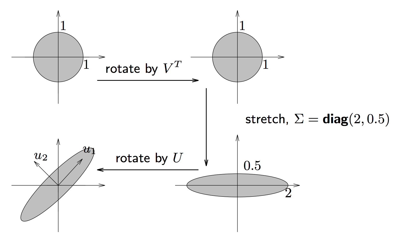
The unit ball is transformed into an ellipsoid. Specifically, \(\{ Ax \mid \|x\| \leq 1 \}\) is an ellipsoid with principal axes \(\sigma_iu_i.\)

SVD Applications

If \(A\) has SVD \(A = U \Sigma V^T\), we can use the SVD to compute the general pseudo-inverse of a matrix:

We substitute in the SVD decomposition of \(A\):

We now wish to find

Since \((AB)^{−1} = B^{−1}A^{−1}\), we can say

Since \(U,V\) are orthogonal matrices, we know \(U^{-1}=U^T\) and \(V^{-1}=V^T\), so

Thus, we have:

Extremal Trace Problems

Eigenvectors

An eigenvector is a vector \(x\) such that

The Sherman-Morrison Formula

Let \(A \in \mathbf{R}^{n \times n}\) (nonsingular) and \(b \in \mathbf{R}^{n \times 1}\). Suppose we wish to solve \(Ax=b\). Although it is a correct procedure to find \(x\) by computing \(x=A^{-1}b\), there exists more efficient solutions. It is not necessary to compute \(A^{-1}\) explicitly.

Assume we already have \(A^{-1}\). However, the matrix \(A\) changed in a very specific way: via a rank-1 update. We now wish to solve the following system:

\((A + uv^T)x = d\).

It turns out that computing the inverse of the new matrix (as long as \(vT A^{−1}u \neq −1\)) is quite easy:

where we call \(uv^T\) the rank-1 update.

Proof: To show that \(B\) is a valid inverse, we must show that \((A + uv^T )B = I\)

Note that \(v^TA^{-1}u\) is a scalar: \((1 \times n)(n \times n)(n \times 1) = (1 \times 1)\).

Sherman-Woodbury-Woodbury Formula

The generalization of the Sherman-Morrison update to a rank-k update from a rank-1 update is called the Sherman-Woodbury-Woodbury Formula.

For example, a rank-2 update is

In general, the update \(A + UV^T\), where \(A \in \mathbf{R}^{n \times n}, U \in \mathbf{R}^{n \times k}, V \in \mathbf{R}^{k \times n}\).

Changing a single matrix entry is a rank-1 update. Consider two matrices, \(A,B\):

As a linear combination of the rows 0 -1 0 )(0 0 1)

As a linear combination of the columns (0 1 0)(0 0 -1)

Perspectives on Matrix Multiplication

Thinking Elementwise Consider two matrices, \(A,B\), where

\(C = A \times B\) \(A \in \mathbf{R}^{m \times n}, B \in \mathbf{R}^{n \times p}\)

Can see \(C_{ij} = \sum\limits_{k=1}^n a_{ik} b_{kj}\)

You can also see it as a sum of many outer products:

or as each element coming from an inner product, i.e. \(C_{ij} = g_i^Tb_j\):

Or get the first row of \(C\), then get the \(j\)‘th column:

References:

These notes are an adaptation of the content taught by Dr. Reza Mahalati in Stanford’s EE 263 course (Linear Dynamical Systems).

1. Duchi, John. Properties of the Trace and Matrix Derivatives.

2. Boyd, Stephen. Linear Dynamical Systems, (EE263) Lecture Slides.

3. Boyd, Stephen. Linear Dynamical Systems, (EE263) Lecture 8: Least-norm solutions of undetermined equations.

4. Zwick. SVD. PDF.